Archive for the 'I/O Topics' Category

Yes, Storage Arrays Can Deduplicate Oracle Database. Here Is Exactly Why It Doesn’t Matter!

I recently had some cycles on a freshly installed Dell EMC XtremIO Storage Array. I took this opportunity to prepare a blog entry about the never-ending topic of whether or not storage arrays are able to reduce physical data capacity through deduplication of blocks in Oracle Database.

Of Course There Is Duplicate Data In Oracle Datafiles

Before I continue, let me say something that may come as a surprise to you. Yes, Oracle Database has duplicate blocks in tablespaces! Yes, modern storage arrays can achieve astonishing data reduction rates through deduplication–even when the only data in the array is Oracle Database (whether ASM or file systems)!

XtremIO computes and displays global data reduction rate. This makes it a bit more difficult to show the effect of deduplication on Oracle Database because averages across diverse data makes pin-point focus impossible. However, as I was saying, I took some time on a freshly-installed XtremIO array and collected what I hope will be interesting information on the topic of deduplication.

Please take a look at Figure 1. To start the testing I created a 4TB XtremIO volume, attached it as a LUN to a test host and then created an XFS file system on it. Please be aware that the contents of an Oracle datafile is precisely the same whether stored in ASM or in a file system file. After the file system was created I used the SLOB database creation kit (SLOB/misc/create_database_kit) to create a small database with Oracle Database 12c. As Figure 1 shows, the small database consumed 11.83GB of logical space in the 4TB volume. However, since the data enjoyed a slight deduplication ratio of 1.1:1 and a healthy compression ratio of 3.3:1 for a 3.6:1 data reduction ratio, only 3.27GB physical space was consumed in the array.

markup-gui-after-slob-database-created

Figure 1

The next step in the testing was to consume the majority of the 4TB file system with a BIGFILE tablespace. Figure 2 shows the DDL I used to create the tablespace.

shell-create-3900g-ts

Figure 2

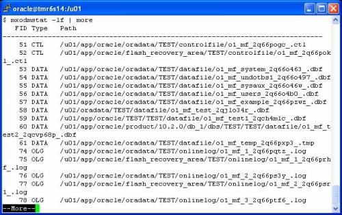
Figure 3 shows the file system file that corresponds to the tablespace created with DDL in Figure 2.

sqlplus-bigfile-info-and-host-to-ls

Figure 3

After creating the 3.9TB BIGFILE tablespace I took a screenshot of the XtremIO GUI Dashboard. As Figure 4 shows, there was no deduplication! Instead, the data was compressed 4.0:1 resulting in only 977.66GB physical space being consumed in the array. So why in the world would I blog the opposite of what I said above? Why show the array did not, in fact, deduplicate the 3.9TB datafile? The answer is in the fact that I said there are duplicate data block in tablespaces. I didn’t say there are duplicate blocks in the same datafile!

gui-after-bigfile-cr

Figure 4

To return the array to the state prior to the BIGFILE tablespace creation, I dropped the tablespace (including contents and datafiles thus unlinking the file) and then used the Linux fstrim(8) command to return the space to the array as shown in Figure 5.

shell-fstrim-after-drop-bigts

Figure 5

Once the fstrim command completed I took another screenshot of the XtremIO GUI Dashboard as shown in Figure 6. Figure 6 shows that the array space utilization and data reduction had returned to that of what was seen before the BIGFILE tablespace creation.
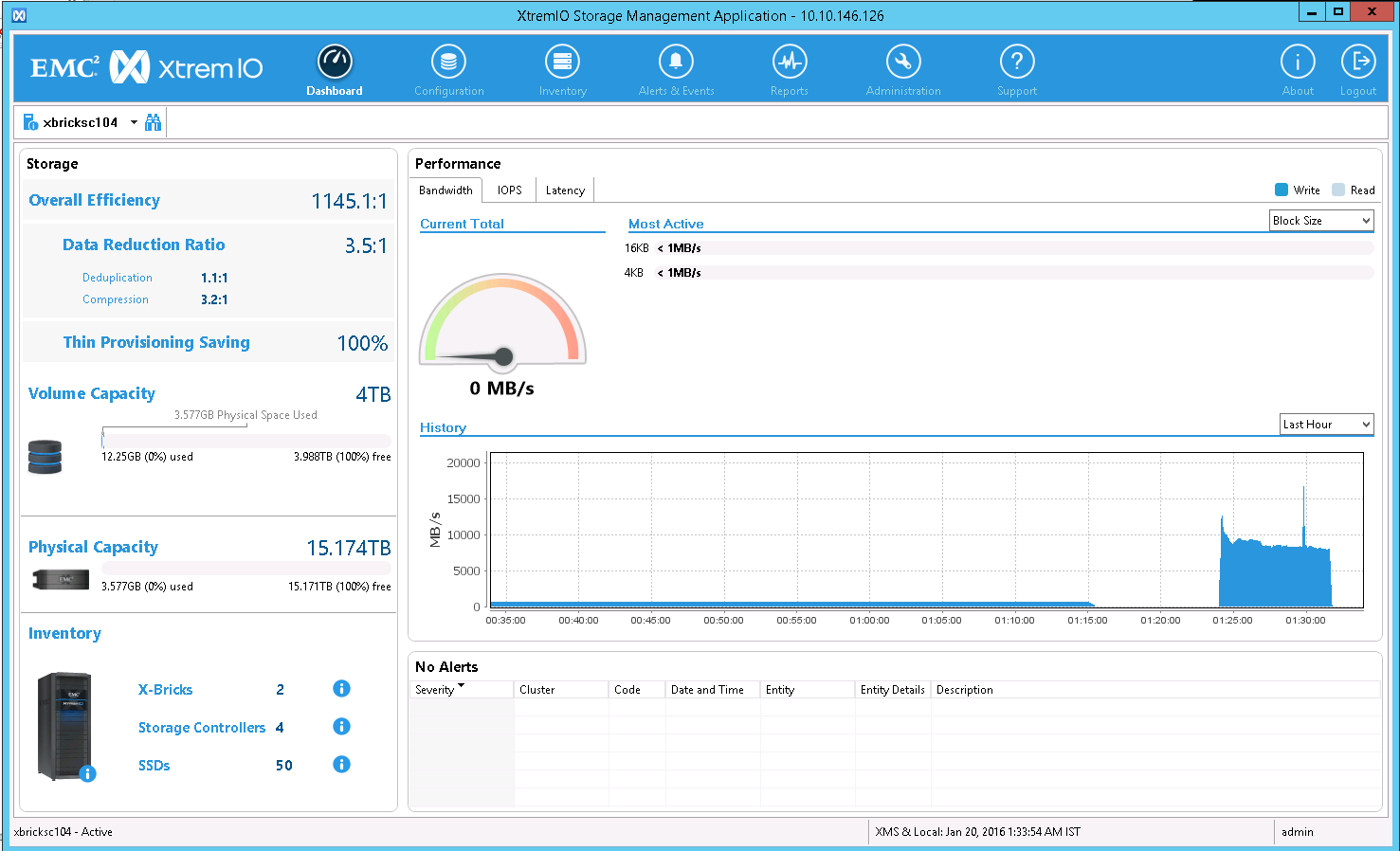
gui-after-bigfile-drop-and-fstrim

Figure 6

OK, Now For The Duplicate Data

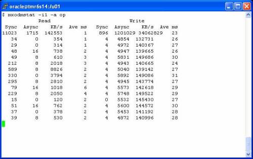
The next step in the testing was to fill up the majority of the 4TB file system with SMALLFILE tablespaces. To do so I created 121 tablespaces each consisting of a single SMALLFILE datafile of 32GB. The output shown in Figure 7 is from a data dictionary query to display the size of each of the 121 datafiles and how the sum of these datafiles consumed 3.87TB of the 4TB file system.

shell-after-creating-smalfile-tablespaces

Figure 7

That’s Duplicate Data

Once the file system was filled with SMALLFILE datafiles I took another screenshot of the XtremIO GUI Dashboard. Figure 8 shows that the SMALLFILE datafiles enjoyed a deduplication ratio 81.8:1 combined with a compression ratio of 3.8:1 resulting in a global data reduction rate of 306.9:1. Because of the significant data reduction rate only 12.68GB of physical space was consumed in the array in spite of the 3.79TB logical space (the sum of the SMALLFILE datafiles) being allocated.

gui-after-smallfile-cr

Figure 8

So here we have it! I had a database created with Oracle Database 12c that consisted of 121 32GB files for roughly 3.8TB database size yet XtremIO deduplicated the data down by a factor of 82:1!

So arrays can deduplicate Oracle Database contents! Right? Well, yes, but it matters none whatsoever. Allow me to explain.

Oracle datafiles consist of initialized blocks but vast portions of that initialized content is the same from file to file. This fact can be seen with simple md5sum(1) output. Consider Figure 9 where you can see the output of the md5sum command used to compute Oracle datafile checksums but only after skipping the first 8,692 blocks (8KB blocks). It’s the first approximate 68MB of each datafile that is unique when a datafile is freshly initialized. Beyond that threshold we can see (Figure 9) that the rest of the file content is identical.
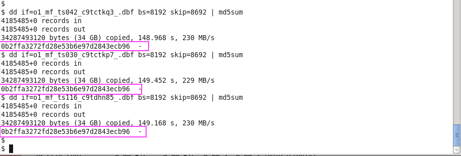
markup-shell-with-md5sum

Figure 9

Thus far this blog post has proven that initialized, but empty, Oracle Database datafiles have duplicate data. As the title of this post says, however, it does not matter.

Introduce Application Data To The Mix

Figure 10 shows the commands I used to populate each of the 121 tablespaces with a single table. The table has the sparse characteristic we are all accustomed to with SLOB. That is, I am only creating a single row in each block. Moreover, I’m populating each of these 121 tables with the same application data! This is precisely why I say deduplication of Oracle Database doesn’t matter because it only holds true until any application data is loaded into the data blocks. Figure 10 shows this set of DDL commands.

shell-load_tablespaces-script

Figure 10

After populating the blocks in each of the 121 tables (each residing in a dedicated SMALLFILE tablespace) with blocks containing just a single row of application data I took another screenshot of the XtremIO GUI Dashboard. Figure 11 shows how putting any data into the data blocks reverts the deduplication. Why? Well, remember that the block header of every block has the SCN of the last change made to the block. For this reason I can put the same application data in blocks and still have 100% unique blocks–at least at the 8KB level.

Please note that the application table I used to populate the 121 tables does not consume 100% of the data blocks in each of the SMALLFILE tablespaces. There were a few blocks remaining in each tablespace and thus there remained a scant amount of deduplication as seen in Figure 11. Most XtremIO customers see some insignificant deduplication in their Oracle Database environments. Some even see significant deduplication–at least until they insert data into the database.
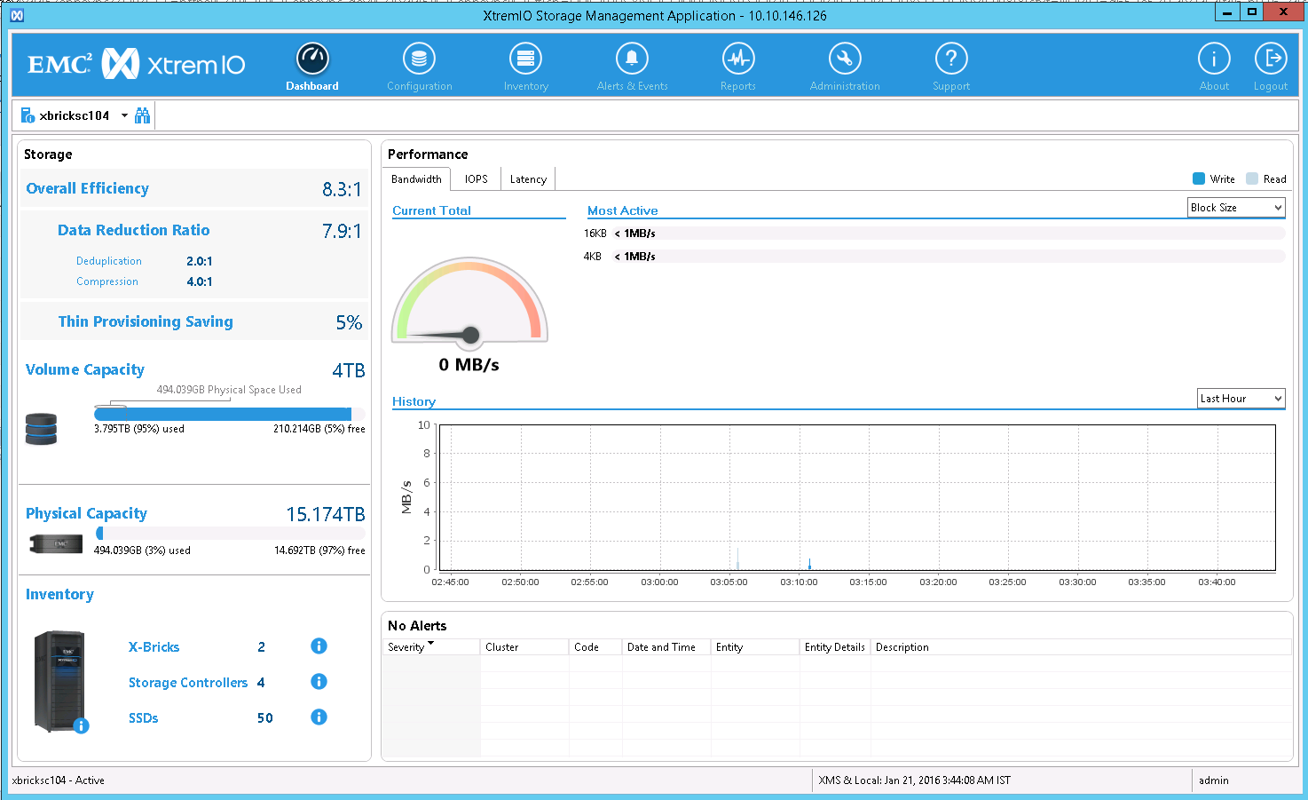
gui-after-filling-smallfiles

Figure 11

In a follow-up post I’ll say a few words about the deduplication granularity and how it affects the ability to achieve small amounts of deduplication of unused space in initialized data blocks. However, bear in mind that the net result of any deduplication of Oracle Database data files is that the only space that can be deduplicated is space that has never had application data in it. After all, a SQL DELETE command doesn’t remove data–it only marks it as free in the block.

Summary

I don’t think there are that many Oracle shops that have an urgent need for data reduction of space that’s never been used to store application data. I could be wrong. Until I find out either way, I say that yes you can see deduplication of Oracle Database datafiles but it doesn’t matter one bit.


EMC XtremIO – The Full-Featured All-Flash Array. Interested In Oracle Performance? See The Whitepaper.

NOTE: There’s a link to the full article at the end of this post.

I recently submitted a manuscript to the EMC XtremIO Business Unit covering some compelling lab results from testing I concluded earlier this year. I hope you’ll find the paper interesting.

There is a link to the full paper at the bottom of this block post. I’ve pasted the executive summary here:

Executive Summary

Physical I/O patterns generated by Oracle Database workloads are well understood. The predictable nature of these I/O characteristics have historically enabled platform vendors to implement widely varying I/O acceleration technologies including prefetching, coalescing transfers, tiering, caching and even I/O elimination. However, the key presumption central to all of these acceleration technologies is that there is an identifiable active data set. While it is true that Oracle Database workloads generally settle on an active data set, the active data set for a workload is seldom static—it tends to move based on easily understood factors such as data aging or business workflow (e.g., “month-end processing”) and even the data source itself. Identifying the current active data set and keeping up with movement of the active data set is complex and time consuming due to variability in workloads, workload types, and number of workloads. Storage administrators constantly chase the performance hotspots caused by the active dataset.

All-Flash Arrays (AFAs) can completely eliminate the need to identify the active dataset because of the ability of flash to service any part of a larger data set equally. But not all AFAs are created equal.

Even though numerous AFAs have come to market, obtaining the best performance required by databases is challenging. The challenge isn’t just limited to performance. Modern storage arrays offer a wide variety of features such as deduplication, snapshots, clones, thin provisioning, and replication. These features are built on top of the underlying disk management engine, and are based on the same rules and limitations favoring sequential I/O. Simply substituting flash for hard drives won’t break these features, but neither will it enhance them.

EMC has developed a new class of enterprise data storage system, XtremIO flash array, which is based entirely on flash media. XtremIO’s approach was not simply to substitute flash in an existing storage controller design or software stack, but rather to engineer an entirely new array from the ground-up to unlock flash’s full performance potential and deliver array-based capabilities that are unprecedented in the context of current storage systems.

This paper will help the reader understand Oracle Database performance bottlenecks and how XtremIO AFAs can help address such bottlenecks with its unique capability to deal with constant variance in the I/O profile and load levels. We demonstrate that it takes a highly flash-optimized architecture to ensure the best Oracle Database user experience. Please read more:  Link to full paper from emc.com.

Oracle Exadata Storage Server: A Black Box with No Statistics.

A question came in about whether it is possible to measure how much data is filtered out when running a query serviced by a Smart Scan in the Exadata Storage Server grid. The following is the long answer.

An Example of Offload Processing Effectiveness Accounting

I’d like to answer this question by taking real information from a test configuration consisting of 4 Real Application Clusters nodes attached to 6 Exadata Storage Server cells with the SAS disk option (12 x 300GB 3.5″ 15K RPM).

Test Workload – The Affinity Card Program Test Database

The Affinity Card Program Test Database (ACPTD) is a test schema and set of queries that mimics the type of queries performed by a marketing group responsible for promoting the use of a retail club card and affinity credit card for a fictitious company. In this example deployment of the ACPTD, the group responsible for promoting club card and affinity credit card activity for Acme Inc has built a data mart with data from several sources, including the main corporate ERP and CRM systems; partner merchant ERP systems; and, outside syndicated data.

For this blog post I’ll focus on the main syndicated card transaction table called all_card_trans. However, there are other tables in the schema and for reference sake the following text box shows the table sizes in my current deployment of the test kit. As the query shows, the all_card_trans table is 613 GB. Yes, I know that’s small, but this is a test system and I don’t like watching 6 Exadata cells hammering 1 GB/s each for tens of minutes when a couple of minutes will do. I hope you’ll understand.

SQL> set echo on
SQL> @tab_sizes
SQL> col segment_name for a32
SQL> select segment_name, sum(bytes)/1024/1024 mb from user_segments
  2  where segment_name not like 'BIN%' and segment_name not like 'SYS%'
  3  group by segment_name;

SEGMENT_NAME                             MB
-------------------------------- ----------
PARTNER_MERCHANTS                         8
PARTNER_MERCHANT_SALES                67780
ZIPCODES                                  8
OUR_SALES                             21956
ALL_CARD_TRANS                       629032
MCC                                       8
OUR_STORES                                8
CUST_SERVICE                             76
TM                                   .03125
CUST_FACT                              4708

10 rows selected.

The table definition for the all_card_trans table is shown in the following text box:

SQL> desc all_card_trans
 Name                                      Null?    Type
 ----------------------------------------- -------- ----------------------------
 CARD_NO                                   NOT NULL VARCHAR2(20)
 CARD_TYPE                                          CHAR(20)
 MCC                                       NOT NULL NUMBER(6)
 PURCHASE_AMT                              NOT NULL NUMBER(6)
 PURCHASE_DT                               NOT NULL DATE
 MERCHANT_CODE                             NOT NULL NUMBER(7)
 MERCHANT_CITY                             NOT NULL VARCHAR2(40)
 MERCHANT_STATE                            NOT NULL CHAR(3)
 MERCHANT_ZIP                              NOT NULL NUMBER(6)

The following queries show the total row count in the all_card_trans table as well as the number of rows representing transactions with credit cards with leading 4 digits of 3333 and 4447, which represent the card block granted to our fictitious company, Acme Inc, for their affinity card program. This is a needle in a haystack query since only .3% of the data matches the where predicate. Now, before you look at the text box please note that this is a single instance of Real Application Clusters driving this query. And, yes, the RAC node is a small 8-core DL360. Both scans are driving storage at 6 GB/s (613GB/102s). Folks, remember that to do what I just did in the following text box with Fibre Channel I’d have to have a system with 15 FC HBAs attached to several huge SAN arrays. Oh, and I should point out that it would also require about 85 Netezza Snippet Processing Units to match this throughput.

SQL> select count(*) from all_card_trans where  card_no like '4777%' or card_no like '3333%’;

  COUNT(*)
----------
  22465830

Elapsed: 00:01:42.71
SQL> select count(*) from all_card_trans;

  COUNT(*)
----------
7897611641

Elapsed: 00:01:42.47

I Can’t Believe I Ate the Whole Thing

The following query uses a method for measuring cell activity by forcing the database to ingest all rows and all columns. Don’t try to make sense of the query because it isn’t supposed to make sense. It is only supposed to drive Exadata to return all rows and all columns, which it does.

$ more demo_offload_bytes.sql

drop view ingest;
create view ingest as
select avg(length(CARD_NO)) c1,
avg(length(CARD_TYPE)) c2,
max(MCC + PURCHASE_AMT) c3,
max(length(PURCHASE_DT)) c4,
max(MERCHANT_CODE) c5,
avg(length(MERCHANT_CITY)) c6,
avg(length(MERCHANT_STATE)) c7,
max(MERCHANT_ZIP) c8 from all_card_trans;

col MB format 99999999.9
select NAME,VALUE/(1024*1024*1024) GB from gv$sysstat where STATISTIC# in (196, 44, 43 );

select c1+c2+c3+c4+c5+c6+c7 from ingest;

select NAME,VALUE/(1024*1024*1024) GB from gv$sysstat where STATISTIC# in (196, 44, 43);

The following text box shows that when I ran the query Exadata (in aggregate) scanned 613 GB of disk and returned all but 6% to the RDBMS instance (delta cell physical IO interconnect bytes). Also recorded by v$sysstat (bytes eligible) is the fact that there was nothing peculiar about the data being scanned-peculiar in any such fashion that would have interfered with offload processing (e.g., chained rows, etc). Since I asked for all the data, that is what I got. It is nice to know, however, that the entirety of the data was a candidate for offload processing.

Notice I didn’t time the query. I’ll offer more on that later in this blog post.

SQL> @demo_offload_bytes

View dropped.

View created.

NAME                                                                     GB
---------------------------------------------------------------- ----------
physical IO disk bytes                                           1227.80814
cell physical IO interconnect bytes                              1151.52453
cell physical IO bytes eligible for predicate offload            1227.31451

C1+C2+C3+C4+C5+C6+C7
--------------------
          9010106.59

NAME                                                                     GB
---------------------------------------------------------------- ----------
physical IO disk bytes                                            1841.5774
cell physical IO interconnect bytes                              1727.15227
cell physical IO bytes eligible for predicate offload            1840.97177

So let’s take a look at some offload processing. The following change to the “ingest” query reduces the amount of data ingested by the database tier by only selecting rows where the credit card number started with 4777 or 3333. We know from the scan of the table that this whittles down the dataset by 99.7%.

$ more demo_offload_bytes1.sql

create view ingest_less as
select avg(length(CARD_NO)) c1,
avg(length(CARD_TYPE)) c2,
max(MCC + PURCHASE_AMT) c3,
max(length(PURCHASE_DT)) c4,
max(MERCHANT_CODE) c5,
avg(length(MERCHANT_CITY)) c6,
avg(length(MERCHANT_STATE)) c7,
max(MERCHANT_ZIP) c8 from all_card_trans act
where card_no like '4777%' or card_no like '3333%';

col MB format 99999999.9
select NAME,VALUE/(1024*1024*1024) GB from gv$sysstat where STATISTIC# in (196, 44, 43 );

set timing on
select c1+c2+c3+c4+c5+c6+c7 from ingest_less;

select NAME,VALUE/(1024*1024*1024) GB from gv$sysstat where STATISTIC# in (196, 44, 43);

The following text box shows that that Exadata scanned and filtered out the uninteresting rows. The projected columns accounted for only 1.7 GB across the iDB intelligent I/O fabric. That is, the database tier only had to ingest 1.7 GB, or 17 MB/s since the query completed in 103 seconds.

SQL> @demo_offload_bytes_1

View dropped.

Elapsed: 00:00:00.21

View created.

Elapsed: 00:00:00.00

NAME                                                                     GB
---------------------------------------------------------------- ----------
physical IO disk bytes                                           1841.13743
cell physical IO interconnect bytes                              43.1782733
cell physical IO bytes eligible for predicate offload            1840.97177

Elapsed: 00:00:00.01

C1+C2+C3+C4+C5+C6+C7
--------------------
           9010106.9

Elapsed: 00:01:43.31

NAME                                                                     GB
---------------------------------------------------------------- ----------
physical IO disk bytes                                           2454.80203
cell physical IO interconnect bytes                              44.8776852
cell physical IO bytes eligible for predicate offload            2454.62903

Elapsed: 00:00:00.00
SQL>

So, yes, Exadata does let you see how effectively Smart Scans are working. In this example we saw a single-table scan on a small Oracle Exadata Storage Server grid weeding out 99.7% of the data.

Sneaky, Sneaky.

You’ll notice when I executed demo_offload_bytes.sql (the non-filtering example) I was not tracking query completion time. That’s because up to this point I’ve only been showing examples driven by a single Real Application Clusters node. Now, let’s think about this. I have 8 Intel processor cores and a single inbound Infiniband path on the database server. From an inbound I/O bandwidth perspective the host can “only” ingest 1.6GB/s, but the CPUs may also further throttle that since the database is doing its own projection in this case.

I’ve shown, in this post, that this test Exadata Storage grid configuration can scan disk at 6 GB/s. The question you might ask-and I’m about to answer-is how much does this single database host throttle storage and why does that matter? Well, it matters because having ample storage bandwidth with limited database server bandwidth is the classic imbalance addressed by the HP Oracle Database Machine. So, let me run it again-with timing turned on. As you’ll see, bottlenecks are bottlenecks. This single database host cannot keep up with storage, so storage is throttled and the result is 18X increase in query completion time when compared to the heavily filtered case. Both queries had to read the same amount of data but in this case there was an imbalance in the upstream ability to ingest the data both from an I/O bandwidth and CPU perspective.

SQL> @demo_offload_bytes

View dropped.

Elapsed: 00:00:00.02

View created.

Elapsed: 00:00:00.01

NAME                                                                     GB
---------------------------------------------------------------- ----------
physical IO disk bytes                                           2454.81084
cell physical IO interconnect bytes                               44.886501
cell physical IO bytes eligible for predicate offload            2454.62903

Elapsed: 00:00:00.00

C1+C2+C3+C4+C5+C6+C7
--------------------
          9010106.59

Elapsed: 00:29:26.85

NAME                                                                     GB
---------------------------------------------------------------- ----------
physical IO disk bytes                                           3068.55792
cell physical IO interconnect bytes                              620.492259
cell physical IO bytes eligible for predicate offload            3068.28629

Elapsed: 00:00:00.00

Need More RDBMS Bandwidth? OK, Use It.

So, let’s see what the full-ingestion case looks like with 4 Real Application Clusters nodes. And please forgive that I forgot to aggregate the v$sysstat output. I’ve added 4-fold database grid resources so I should complete the full-ingestion query in 75% less time. The text box starts out showing that the number of RAC instances was increased from 1 to 4.

SQL> host date
Fri Oct  3 16:27:52 PDT 2008

SQL> select instance_name from gv$instance;

INSTANCE_NAME
----------------
test1

Elapsed: 00:00:00.02
SQL> select instance_name from gv$instance;

INSTANCE_NAME
----------------
test1
test4
test3
test2

Elapsed: 00:00:00.08
SQL> host date
Fri Oct  3 16:32:06 PDT 2008
SQL>
SQL> @demo_offload_bytes

View dropped.

Elapsed: 00:00:00.03

View created.

Elapsed: 00:00:00.01

NAME                                                                     GB
---------------------------------------------------------------- ----------
physical IO disk bytes                                           3068.69843
cell physical IO interconnect bytes                              620.632769
cell physical IO bytes eligible for predicate offload            3068.28629
physical IO disk bytes                                           .013385296
cell physical IO interconnect bytes                              .013385296
cell physical IO bytes eligible for predicate offload                     0
physical IO disk bytes                                           .010355473
cell physical IO interconnect bytes                              .010355473
cell physical IO bytes eligible for predicate offload                     0
physical IO disk bytes                                           .031275272
cell physical IO interconnect bytes                              .031275272

NAME                                                                     GB
---------------------------------------------------------------- ----------
cell physical IO bytes eligible for predicate offload                     0

12 rows selected.

Elapsed: 00:00:00.02

C1+C2+C3+C4+C5+C6+C7
--------------------
          9010106.59
Elapsed: 00:07:25.01

NAME                                                                     GB
---------------------------------------------------------------- ----------
physical IO disk bytes                                           3222.13893
cell physical IO interconnect bytes                              764.535856
cell physical IO bytes eligible for predicate offload            3221.70425
physical IO disk bytes                                            154.31714
cell physical IO interconnect bytes                              144.732708
cell physical IO bytes eligible for predicate offload            154.280945
physical IO disk bytes                                           152.860648
cell physical IO interconnect bytes                              143.367385
cell physical IO bytes eligible for predicate offload            152.828033
physical IO disk bytes                                           153.195674
cell physical IO interconnect bytes                                143.6831

NAME                                                                     GB
---------------------------------------------------------------- ----------
cell physical IO bytes eligible for predicate offload             153.13031

12 rows selected.

Elapsed: 00:00:00.02
SQL>

Well, that was predictable, but cool nonetheless. What about the filtered ingest-query? Should there be much of a speedup given the fact that storage bandwidth remains constant and the ingest rate of the filtered query was only roughly 17 MB/s with a single Real Application Clusters node? I could save the cut and paste effort and just tell you that adding Real Application Clusters nodes in this case will, of course, not reduce the query time, but since I’ve bored you this long, here it is:

SQL> @demo_offload_bytes_1

View dropped.

Elapsed: 00:00:00.01

View created.

Elapsed: 00:00:00.01

NAME                                                                     GB
---------------------------------------------------------------- ----------
physical IO disk bytes                                           3222.15758
cell physical IO interconnect bytes                              764.554509
cell physical IO bytes eligible for predicate offload            3221.70425
physical IO disk bytes                                           154.334342
cell physical IO interconnect bytes                               144.74991
cell physical IO bytes eligible for predicate offload            154.280945
physical IO disk bytes                                           153.213285
cell physical IO interconnect bytes                               143.70071
cell physical IO bytes eligible for predicate offload             153.13031
physical IO disk bytes                                           152.878347
cell physical IO interconnect bytes                              143.385084

NAME                                                                     GB
---------------------------------------------------------------- ----------
cell physical IO bytes eligible for predicate offload            152.828033

12 rows selected.

Elapsed: 00:00:00.01

C1+C2+C3+C4+C5+C6+C7
--------------------
           9010106.9

Elapsed: 00:01:42.79

NAME                                                                     GB
---------------------------------------------------------------- ----------
physical IO disk bytes                                           3375.27835
cell physical IO interconnect bytes                              764.974159
cell physical IO bytes eligible for predicate offload            3374.81995
physical IO disk bytes                                             308.0746
cell physical IO interconnect bytes                              144.133529
cell physical IO bytes eligible for predicate offload            307.986572
physical IO disk bytes                                           310.634206
cell physical IO interconnect bytes                              145.189768
cell physical IO bytes eligible for predicate offload              310.5755
physical IO disk bytes                                           302.274069
cell physical IO interconnect bytes                              143.805239

NAME                                                                     GB
---------------------------------------------------------------- ----------
cell physical IO bytes eligible for predicate offload            302.218781

12 rows selected.

Elapsed: 00:00:00.01
SQL> host date
Fri Oct  3 16:49:32 PDT 2008

Summary

Exadata works and has statistics so that the solution doesn’t feel so much like a black box. In the end, however, none of the statistcs stuff really matters. What matters is whether your queries complete in the desired service times.

Oracle Exadata Storage Server Version 1. A “FAQ” is Born. Part I.

BLOG UPDATE (22-MAR-10): Readers, please be aware that this blog entry is about the HP Oracle Database Machine (V1).

BLOG UPDATE (01-JUN-09). According to my blog statistics, a good number of new readers find my blog by being referred to this page by google. I’d like to draw new readers’ attention to the sidebar at the right where there are pages dedicated to indexing my Exadata-related posts.  The original blog post follows:

I expected Oracle Exadata Storage Server to make an instant splash, but the blogosphere has really taken off like a rocket with the topic. Unfortunately there is already quite a bit of misinformation out there. I’d like to approach this with routine quasi-frequently asked question posts. When I find misinformation, I’ll make a blog update. So consider this installment number one.

Q. What does the word programmable mean in the product name Exadata Programmable Storage Server?

A. I don’t know, but it certainly has nothing to do with Oracle Exadata Storage Server. I have seen this moniker misapplied to the product. An Exadata Storage Server “Cell”-as we call them-is no more programmable than a Fibre Channel SAN or NAS Filer. Well, it is of course to the Exadata product development organization, but there is nothing programmable for the field. I think, perhaps, someone may have thought that Exadata is a field programmable gate array (FPGA) approach to solving the problem of offloading query intelligence to storage. Exadata is not field-“programmable” and it doesn’t use or need FPGA technology.

Q. How can Exadata be so powerful if there is only a single 1gb path from the storage cells to the switch?

A. I saw this on a blog post today and it is an incorrect assertion. In fact, I saw a blogger state, “1gb/s???? that’s not that good.” I couldn’t agree more. This is just a common notation blunder. There is, in fact, 20 Gb bandwidth between each Cell and each host in the database grid, which is close to 2 gigabytes of bandwidth (maximum theoretical 1850MB/s due to the IB cards though). I should point out that none of the physical plumbing is “secret-sauce.” Exadata leverages commodity components and open standards (e.g., OFED ).

Q. How does Exadata change the SGA caching dynamic?

A. It doesn’t. Everything that is cached today in the SGA will still be cached. Most Exadata reads are buffered in the PGA since the plan is generally a full scan. That is not to say that there is no Exadata value for indexes, because there can be. Exadata scans indexes and tables with the same I/O dynamic.

Q. This Exadata stuff must be based on NAND FLASH Solid State Disk

A. No, it isn’t and I won’t talk about futures. Exadata doesn’t really need Solid State Disk. Let’s think this one through. Large sequential read and write  speed is about the same on FLASH SSD as rotating media, but random I/O is very fast. 12 Hard Disk Drives can saturate the I/O controller so plugging SSD in where the 3.5″ HDDs are would be a waste.

Q. Why mention sequential disk I/O performance since sequential accesses will only occur in rare circumstances (e.g., non-concurrent scans).

A. Yes, and the question is what? No, honestly. I’ll touch on this. Of course concurrent queries attacking the same physical disks will introduce seek times and rotational delays. And the “competition” can somehow magically scan different table extents on the same disks without causing the same drive dynamic? Of course not. If Exadata is servicing concurrent queries that attack different regions of the same drives then, yes, by all means there will be seeks. Those seek, by the way, are followed by 4 sequential 1MB I/O operations so the seek time is essentailly amortized out.

Q. Is Exadata I/O really sequential, ever?

A. I get this one a lot and it generally comes from folks that know Automatic Storage Management (ASM). Exadata leverages ASM normal redundancy mirroring which mirrors and stripes the data. Oh my, doesn’t that entail textbook random I/O? No, not really. ASM will “fill” a disk from the “outside-in. ” This does not create a totally random I/O pattern since this placement doesn’t randomize from the outer edge of the platters to the spindle and back. In general, the “next” read on any given disk involved in a scan will be at a greater offset in the physical device and not that “far” from the previous sectors read. This does not create the pathological seek times that would be associated with a true random I/O profile.

When Exadata is scanning a disk that is part of an ASM normal redundancy disk group and needs to “advance forward” to get the next portion of the table, Exadata directs the drive mechanics to position at the specific offset where it will read an ASM allocation unit of data, and on and on it goes. Head movements of this variety are considered “short seeks.” I know what the competition says about this topic in their positioning papers. Misinformation will be propagated.

Let me see if I can handle this topic in a different manner. If HP Oracle Exadata Storage Server was a totally random I/O train wreck then it wouldn’t likely be able to drive all the disks in the system at ~85MB/s. In the end, I personally think the demonstrated throughput is more interesting than an academic argument one might stumble upon in an anti-Exadata positioning paper.

Well, I think I’ll wrap this up as installment one of an on-going thread of Q&A on HP Oracle Exadata Storage Server and the HP Oracle Database Machine.

Don’t forget to read Ron Weiss’ Oracle Exadata Storage Server Technical Product Whitepaper. Ron is a good guy and it is a very informative piece. Consider it required reading-especially if you are trolling my site in the role of competitive technical marketing. <smiley>

Manly Men Only Deploy Oracle with Fibre Channel – Part V. What About Oracle9i on RHAS 2.1? Yippie!

Due to my Manly Man Fibre Channel Series Part I , Part II , Part III and Part IV, my email box is getting loaded with a lot of questions about various Oracle over NFS combinations. The questions run the gamut from how to best tune Oracle9i on Red Hat AS 2.1 to Oracle10g on Red Hat RHEL 3 (all on NAS/NFS of course). And then it dawned on me. When I say I’m a fan of Oracle over NFS, that is just entirely too generic.

It Ain’t Linux Unless It Is a 2.6 Kernel
Honestly folks, Red Hat 3.0-or worse yet, RHAS 2.1? Sheer madness. I’m more than convinced that there are a lot of solid RHEL 3.0 systems out there running Oracle. To those folks I’d say, “If it isn’t broken, don’t fix it.” But RHAS 2.1? That wasn’t even an operating system and to be hyper-critically honest, the “franken-kernel” that was RHEL 3.0 wasn’t really that much better, what with that hugemem 4×4 split garbage and all. SuSE SLES8 was vastly more stable than RHEL 3.0. But I digress. Look, if you are running on a pre-2.6 Kernel Linux distribution you’ve simply got to do yourself a favor and plan an upgrade! Now, back to NAS.

What Oracle on NFS?
I’ll be brief, I wouldn’t even think about using Oracle9i on NAS. I know there are a ton of databases out there doing it, but that is just me. The Oracle Server code specific to NFS (Operating System Dependent code) has gone through some serious evolution/maturation. I’ve watched the changes specifically handling NFS mature from 9i through 10g and now into 11g. Simply put, I didn’t like what I say in Oracle9i-specific to NFS that is. Oracle9i is a perfectly fine release-albeit the port to 64bit Linux was pretty scary. I guess I wasn’t that brief. So I’ll continue.

So, Oracle9i on NAS is a no-go (in my book), what about Oracle10g? There again, I’ll be brief. In my opinion, Oracle10gR1 on NAS was about as elegant as a fish flopping around on a hot sidewalk-not a pretty picture. Yes, I have my reasons why for all this stuff, but this blog entry is purely an assertion of my opinion.

Thus far, I discussed 9i and 10gR1 Linux ports. I cannot speak authoritatively about the Solaris ports of either vis a vis fitness for NFS. If I was a betting man and had two dimes to rub together I would wager them that even the Solaris releases of 9i and 10g were probably pretty shaky on NAS. That leads us to 10gR2.

Solid
Oracle10gR2 on NAS is solid-at least for Linux clients. I have seen Metalink stories about Legacy Unix ports that have RMAN problems with NFS as a near-line backup target. Again, I cannot speak for all these sundry platforms. They are good platforms, but I don’t deal with them day to day.

11g
Don’t jump the gun…tomorrow AM…

Examples
In this May 5, 2007 post on toasters, a list participant posted the following:

We are about to start testing Oracle 9i (single instance) with NetApp NAS (6070) filers. We currently have Oracle running on Solaris 9 with SAN storage attached and VERITAS.

I wouldn’t touch that project with a 10 foot pole. If that database is stable, I wouldn’t switch out the storage architecture-especially on that old of an Oracle release.

I’ve also had a thread going with Chen Shapira who has blogged about Oracle troubles on NAS. Her point throughout that blog entry, and the comments to follow, was that they’ve suffered uptime impact that never really solidly indicts to the storage, but there seems to be a lot of fingers pointed that way. Having read of the types of instability his systems have suffered, I suspected old stuff. It came out in the comment section that they are on RHEL 3.0 64-bit. Now, like I’ve said, RHEL 3.0 is carrying a lot of Oracle databases out there I know, but I wonder how many on NAS? When I say Oracle on NFS, I’m mostly saying Linux Oracle10gR2 releases on Linux 2.6 Kernels—and beyond.

I made a blog entry on this topic back in October of last year as well.

Old Operating System Releases
I take criticism (by true believers mostly) when I point out that running Oracle on a Legacy Unix release that is, say, four years old is not a reason for concern. I wish I could say the same thing about the current state of the art in the Linux world. Dating back to my first high-end Linux project (The Tens–A 10 Node, 10TB, 10,000 User Oracle9i Linux Cluster Project in 2002), I’ve been routinely reminded that Linux stands for:

(L)inux (i)s (n)ot (u)ni(x)

Now, that said, you’ll find much less dissatisfaction with Oracle in general on 2.6 Linux Kernel based systems, but in my opinion, that goes extra for NAS deployments

SAN Admins: Please Give Me As Much Capacity From As Few Spindles As Possible!

I was catching up on my mojo reading when I caught a little snippet I’d like to blog about. Oh, by the way, have I mentioned recently that StorageMojo is one of my favorite blogs?

In Robin Harris’ latest installment about ZFS action at Apple, he let out a glimpse of one of his other apparent morbid curiosities—flash. Just joking, I don’t think ZFS on Mac or flash technology are morbid, it just sounded catchy. Anyway, he says:

I’ve been delving deep into flash disks. Can you say “weird”? My take now is that flash drives are to disk drives what quantum mechanics is to Newtonian physics. I’m planning to have something out next week.

I look forward to what he has to say. I too have a great interest in flash.

Now, folks, just because we are Oracle-types and Jim Grey was/is a Microsoft researcher, you cannot overlook what sorts of things Jim was/is interesting in. Jim’s work has had a huge impact on technology over the years and it turns out that Jim took/takes an interest in flash technology with servers in mind. Just the abstract of that paper makes it a natural must-read for Oracle performance minded individuals. Why? Because it states (with emphasis added by me):

Executive summary: Future flash-based disks could provide breakthroughs in IOps, power, reliability, and volumetric capacity when compared to conventional disks.


Yes, IOps! Nothing else really matter where Oracle database is concerned. How can I say that? Folks, round-brown spinning things do sequential I/O just fine—naturally. What they don’t do is random I/O. To make it worse, most SAN array controllers (you know, that late 1990’s technology) pile on overhead that further choke off random I/O performance. Combine all that with the standard IT blunder of allocating space for Oracle on a pure capacity basis and you get the classic OakTable Network response:

Attention DBAs, it’s time for some déjà vu. I’ll state with belligerent repetition, redundantly, over and over, monotonously reiterating this one very important recurrent bit of advice: Do everything you can to get spindles from your storage group—not just capacity.


Flash
Yes that’s right, it wont be long (in relative terms) until you see flash memory storage fit for Oracle databases. The aspect of this likely future trend that I can’t predict, however, is what impact such technology would have on the entrenched SAN array providers. Will it make it more difficult to keep the margins at the levels they demand, or will flash be the final straw that commoditizes enterprise storage? Then again, and Jim Grey points out in that paper, flash density isn’t even being driven by the PC—and most certainly not enterprise storage—ecosystem. The density is being driven by consumer and mobile applications. Hey, I want my MTV. Um, like all of it, crammed into my credit-card sized mpeg player too.

When?
When it gets cheaper and higher capacity of course. Well, its not exactly that simple. I went spelunking for that Samsung 1.8” 32GB SSD and found two providers with street price of roughly USD $700.00 for 32GB here and here. In fact, upon further investigation, Ritek may soon offer a 32GB device at some $8 per GB. But let’s stick with current product for the moment. At $22 per GB, we’re not exactly talking SATA which runs more on the order of $.35 per GB. But then we are talking enterprise applications here, so a better comparison would be to Fibre drives which go for about $3-$4 per GB.

Now that is interesting since Jim Grey pointed out that in-spite of some industry predictions setting the stage for NAND to double every year, NAND had in fact gained 16 fold in 4 years–off by year. If that pace continues, could we really expect 512GB 1.8″ SSD devices in the next 4 years? And would the price stay relatively constant yielding a cost of something like $1.35 per GB? Remember, even the current state of the art (e.g., the Samsung 1.8″ 32GB SSD) delivers on the order of 130,000 random single-sector IOps–that’s approximately 7usec latency for a random I/O. At least that is what Samsung’s literature claims. Jim’s paper, on the other hand reports grim current art performance when measured with DskSpd.exe:

The story for random IOs is more complex – and disappointing. For the typical 4-deep 8KB random request, read performance is a spectacular 2,800 requests/second but write performance is a disappointing 27 requests/second.

The technology is young and technically superior, but there is work to do in getting the most out of NSSD as the paper reports. Jim suspects that short term quick fixes could be made to bring the random I/O performance for 8KB transfers on today’s NSSD technology up to about 1,700 IOps split evenly between read and write. Consider, however, that real world applications seldom exhibit a read:write ratio of 50:50. Jim generalized on the TPC-C workload as a case in point. It seems with “some re-engineering” (Jim’s words) even today’s SSD would be a great replacement for hard drives for typical Oracle OLTP workloads since you’ll see more 70:30 read:write ratios in the real world. And what about sequential writes? Well, there again, even today’s technology can handle some 35MB/s of sequential writes so direct path writes (e.g., sort spills) and redo log writes would be well taken care of. But alas, the $$/GB is still off. Time will fix that problem and when it does, NSSD will be a great fit for databases.

Don’t think for a moment Oracle Corporation is going to pass up on enabling customers to exploit that sort of performance–with or without the major SAN vendors.

But flash burns out, right? Well, yes and no. The thing that matters is how long the device lasts-the sum of its parts. MTBF numbers are crude, but Samsung sticks a 1,000,000hr MTBF on this little jewel-how cool.
Well, I’ve got the cart well ahead of the horse here for sure because it is still too expensive, but put it on the back burner, because we aren’t using Betamax now and I expect we’ll be using fewer round-brown spinning things in the span of our careers.

Apple OS/X with ZFS Shall Rule the World.

The problem with blogging is there is no way to clearly write something tongue-in-cheek. No facial expressions, no smirking, no hand waving—just plain old black and white. That aside, I can’t resist posting a follow-up to a post on StorageMojo about ZFS performance. I’m not taking a swipe at StorageMojo because it is one of my favorite blogs. However, every now and again third party perspective is a healthy thing. The topic at hand is this post about ZFS performance which is a digest of this post on digitalbadger.net. The original post starts with:

I have seen many benchmarks indicating that for general usage, ZFS should be at least as fast if not faster than UFS (directio not withstanding)[…]

Right off the bat I was scratching my head. I have experience with direct I/O dating back to 1991 and have some direct I/O related posts here. I was trying to figure out what the phrase “directio not withstanding” was supposed to mean. The only performance boost direct I/O can possibly yield is due to the elimination of the write-ordering locks generally imposed by POSIX and the double-buffering/memcopys overhead associated with the DMA into the page cache—and subsequent copy into the user address space buffer. So for a read-intensive benchmark, about the only thing one should expect is less processor overhead, not increased throughput.

Anyway, the post continues:

To give a little background : I have been experiencing really bad throughput on our 3510-based SAN. The hosts are X4100s, 12Gb RAM, 2x dual core 2.6Ghz opterons and Solaris 10 11/06. They are each connected to a 3510FC dual-controller array via a dual-port HBA and 2 Brocade SW200e switches, using MxPIO. All fabric is at 2Gb/s […]

OK, the 4100 is a 2-way Opteron 2000 server which, being a lot like an HP Proliant DL385, should have no problem consuming all the data the 2 x 2Gb FCP paths can deliver—roughly 400MB/s. If the post is about a UFS versus ZFS apples-apples comparison, both results should top out at the maximum theoretical throughput of 2x2Gb FCP. The post continues:

On average, I was seeing some pretty average to poor rates on the non-ZFS volumes depending on how they were configured, on average I was seeing 65MB/s write performance and around 450MB/s read on the SAN using a single drive LUN.

I’d be plenty happy with that 450MB/s given that configuration. The post insinuates this is direct I/O so getting 450MB/s out of 2x2Gb FCP should be the end of the contest. Further, getting 65MB/s written to a single drive LUN is quite snappy! What is left to benchmark? It seems UFS cranks the SAN at full bandwidth.

The post continues:

I then tried ZFS, and immediately started seeing a crazy rate of around 1GB/s read AND write, peaking at close to 2GB/s. Given that this was round 2 to 4 times the capacity of the fabric, it was clear something was going awry.

Hmmm…Opterons with HT 2.0 attaining peaks of 2GB/s write throughput via 2x2Gb FCP? There is nothing awry about this, it is simply not writing the data to the storage.

This is a memory test. ZFS is caching, UFS is not.

The post continues:

Many thanks to Greg Menke and Tim Bradshaw on comp.unix.solaris for their help in unravelling this mystery!

What mystery? I’d recommend testing something that runs longer than 1 second (reading 512MB from memory on any Opteron system should take about .6 seconds. I’d recommend a dataset that is about 2 fold larger than physical memory.

How Does ZFS and UFS Compare to Other Filesystems?
Let’s take a look at an equivalent test running on the HP Cluster Gateway internal filesystem (the former PolyServe PSFS). The following is a screen shot of a dd(1) test using real Oracle datafiles on a Proliant DL585. The first test executes a single thread of dd(1) reading the first 512MB of one of the files using 1M read requests. The throughput is 815MB/s. Next, I ran 2 concurrent dd(1) processes each chomping the first 512MB out of two different Oracle datafiles using 1MB read requests. In the concurrent case, the throughput was 1.46GB/s.

NOTE: You may have to right click->view the image.

zfsthing1.jpg

But wait, in order to prove the vast superiority of the HP Cluster Gateway filesystem over ZFS using similar hardware, I fired off 6 concurrent dd(1) processes each reading the first 512MB out of six different files. Here I measured 2.9GB/s!

zfsthing2.jpg

SAN Array Cache and Filers Hate Sequential Writes

Or at least they should.

Jonathan Lewis has taken on a recent Oracle-l thread about Thinking Big. It’s a good blog entry and I recommend giving it a read. The original Oracle-l post read like this:

We need to store apporx 300 GB of data a month. It will be OLTP system. We want to use 
commodity hardware and open source database. we are willing to sacrifice performance 
for cost. E.g. a single row search from 2 billion rows table should be returned in 2 sec.

I replied to that Oracle-l post with:

Try loading a free Linux distro and typing :
man dbopen
man hash
man btree
man mppo
man recno

Yes, I was being sarcastic, but on the other hand I have been involved with application projects where we actually used these time-tested “database” primitives…and primitive they are! Anyway, Jonathan’s blog entry actually took on the topic and covers some interesting aspects. He ends with some of the physical storage concepts that would likely be involved. He writes:


SANs can move large amounts of data around very quickly – but don’t work well with very large numbers of extremely random I/Os. Any cache benefit you might have got from the SAN has already been used by Oracle in caching the branch blocks of the indexes. What the SAN can give you is a write-cache benefit for the log writer, database writer, and any direct path writes and re-reads from sorting and hashing.

Love Your Cache, Hate Large Sequential Writes
OK, this is the part about which I’d like to make a short comment—specifically about Log Writer. It turns out that most SAN arrays don’t handle sequential writes well either. All told, arrays shouldn’t be in the business of caching sequential writes (yes, there needs to be a cut-off there somewhere). I’ve had experiences with some that don’t cache sequential writes and that is generally good. I’ve had experiences with a lot that do and when you have a workload that generates a lot of redo, LGWR I/O can literally swamp an array cache. Sure, the blocks should be cached long enough for the write back to disk, but allowing those blocks to push into the array cache any further than the least of the LRU end makes little sense. Marketing words for arrays that handle these subtleties usually sound like, “Adaptive Array Cache”, or words to that effect.

One trick that can be used to see such potential damage is to run your test workload with concurrent sequential write “noise.” If you create a couple of files the same size as your redo logs and loop a couple of dd(1) processes performing 128K writes—without truncating the files on open—you can drive up this sort of I/O to see what it does to the array performance. If the array handles the caching of sequential writes, without polluting the cache, you shouldn’t get very much damage. An example of such a dd(1) command is:

$ dd if=/dev/zero of=pseudo_redo_file_db1 bs=128k count=8192 conv=notrunc &

$ dd if=/dev/zero of=pseudo_redo_file_db2 bs=128k count=8192 conv=notrunc &

$ wait

Looping this sort of “noise workload” will simulate a lot of LGWR I/O for two databases. Considering the typical revisit rate of the other array cache contents, this sort of dd(1) I/O shouldn’t completely obliterate your cache. If it does, you have an array that is too fond of sequential writes.

What Does This Have To Do With NAS?
This sort of workload can kill a filer. That doesn’t mean I’m any less excited about Oracle over NFS—I just don’t like filers. I recommend my collection of NFS related posts and my Scalable NAS for Oracle paper for background on what sequential writes can do to certain NAS implementations.

I’ll be talking about this topic and more at Utah Oracle User Group on March 21st.


Standard File System Tools? We Don’t Need No Standard File System Tools!

Yesterday I posted a blog entry about copying files on Solaris. I received some side channel email on the post such as one with the following tidbit from a very good, long time friend of mine. He wrote:

So optimizing cp() is now your hobby? What’s next….. “ed”… no wait “df”.. boy it sure would be great if I could get a 20% improvement in “ls”… I am sure these commands are limiting the number of orders/hr my business can process :)))

Didn’t that blog entry show a traditional cp(1) implementation utilizing 26% less kernel mode processor cycles? Oh well.

It’s About the Whole System
While those were words spoken in jest, it warrants a blog entry and I’ll tell you why. It is true this is an Oracle related blog and such filesystem tools as cp(1) are not in the Oracle code path. I blog about these things for two reasons: 1) a lot of my readers enjoy learning more about the platform in general and 2) many—perhaps most—Oracle systems have normal file system tools such as cp(1), compress(1) and others running while Oracle is running. For that matter, the Oracle server can call out to the same libraries these tools use for such functionality as BFILE and UTL_FILE. For that reason, I feel these topics are related to Oracle platforms. After all, a garbage-can implementation of the standard filesystem tools—and/or the kernel code paths that service them—is going to take cycles away from Oracle. Now please don’t quote me as saying the mmap()-enabled Solaris cp(1) is a “garbage-can” implementation. I’m just making the point that if such tools are implemented poorly Oracle can be affected even though they are not in the scope of a transaction. It’s about the whole system.

Legacy Code. What Comes Around…Stays Around.
Let’s not think for even a moment that the internals of such tools as ls(1) and df(1) are beyond scrutiny. Both ls(1) and df(1) use the stat(2) system call. We Oracle-minded folks often forget that there is much more unstructured data than structured so it is a good thing there are still some folks like PolyServe (HP) minding the store for the performance of such mundane topics as stat(2). Why? Well, perfect examples are the online photo operations such as Snapfish. Try having thousands of threads accessing tens of millions of files (photos) for fun. See, Snapfish uses the HP Enterprise File Services Clustered Gateway NAS powered by PolyServe. You can bet we pay attention to “mundane” topics like what ls(1) behaves like in a directory with 1, 2 or 100 million small files. The stat(2) system call is extremely important in such situations.

He’s Off His Rocker—This is an Oracle Blog.
What could this possibly have to do with Oracle? Well, if you run Oracle on a platform that only specializes in the code underpinnings of the most common server I/O (e.g., db file sequential read, db file scattered read, direct path read/write, LGWR and DBWR writes), you might not end up very happy if you have to do things that hammer the filesystem with Oracle features like UTL_FILE, BFILE, external tables, imp/exp and so forth, cp(1), tar(1), compress(1) and so on. It’s all about taking a holistic view instead of “camps” that focus on segments of the I/O stack.

As the cliché goes, standard file operations and highly specialized Oracle code paths are often joined at the hip.

Copying Files on Solaris. Slow or Fast, It’s Your Choice. Part I

In my recent blog post entitled Standard File Utilities with Direct I/O, I covered the concept of using direct I/O filesystems for storing files to eliminate the overhead of caching them. Consider such files as archived redo. It makes no sense polluting memory with spooled archived redo logs. Likewise, if you compress archived redo it makes little sense to have those disk blocks hanging out in main memory. However, the thread discusses the fact that most operating system file tools do their work by issuing ridiculously small I/O requests. If you haven’t yet, I encourage you to read that blog entry.

The blog entry seeded a lively thread of comments—some touched on theory, others were evidence of entirely missing the point. One excellent comment came in that refreshed some long-lost memories of Solaris. The reader wrote:

For what its worth, cp on Solaris 10 uses mmap64 in 8MB chunks to read in data and 8MB write()s to write it out.

I did in fact know that but it had been a while since I have played around on Solaris.

The Smell Test
I wasn’t fortunate enough to have genius passed to me through genetics. Oh how it seems life would be simpler if that were the case. But it isn’t. So, my motto is, “99% Perspiration, 1% Inspiration.” To that end, I learned early on in my career to develop the skills needed to spot something that cannot be correct—before bothering myself with whether or not it is in fact correct. There is a subtle difference. As soon as the Solaris mmap() enabled cp(1) thing cropped up, I spent next to no time at all pondering how that must certainly be better than normal reads (e.g., pread()) since it failed my smell test.

Ponder Before We Measure
What did I smell? There is just no way that walking through the input file by mapping, unmapping and remapping 8MB at a time could be faster than simply reusing a heap buffer. No way at all. After all, mmap() has to make VM adjustments that are not exactly cheap so taxing every trip to disk with a vigorous jolt of VM overhead makes little sense.

There must have been some point in time when a cp(1) implemented with mmap() was faster, but I suspect that was long ago. For instance, perhaps back in the day before pread(1)/pwrite(). Before these calls, positioning and reading a file required 2 kernel dives (one to seek and the other to read). Uh, but hold it. We are talking about cp(1) here—not random reads—where each successful read on the input file automatically adjusts the file pointer. That is, the input work loop would never have been encumbered with a pair of seek and read. Hmmm. Anyway, we can guess all day long why the Solaris folks chose to have cp(1) use mmap(2) as its input work horse, but in the end we’ll likely never know.

A Closer Look
In the following truss output, the Solaris cp(1) is copying a 5.8MB file to an output file called “xxx.” After getting a file descriptor for the input file, the output file is created. Next, mmap() is used on the input file (reading all 5.8MB since it is smaller than the 8MB operation limit). Next, the write call is used to write all 6161922 bytes from the mmap()ed region out to the output file (fd 4).

open64("SYSLOG-4", O_RDONLY) = 3
creat64("xxx", 0777) = 4
stat64("xxx", 0x00028640) = 0
fstat64(3, 0x000286D8) = 0
mmap64(0x00000000, 6161922, PROT_READ, MAP_SHARED, 3, 0) = 0xFEC00000
write(4, " F e b 5 1 0 : 3 6".., 6161922) = 6161922
munmap(0xFEC00000, 6161922) = 0

Of course if the file happened to be larger than 8MB, cp(1) would unmap and then remap the next chunk and on it would proceed in a loop until the input EOF is reached. That is a lot more “moving parts” than simply calling read(2) over and over clobbering the contents of a buffer allocated at the onset of the copy operation—without continual agitation of the VM subsystem with mmap().

I couldn’t imagine how cp(1) using mmap() would be any faster than read(2)/write(2). But then, it actually only replaces the input read with an mmap() while using write(2) on the output side. I couldn’t imagine how replacing just the input portion with mmap() would be faster than a cp() that uses a static heap buffer with read/write pairs. Moreover, I couldn’t picture how the mmap() approach would be easier on resources.

Measure Before Blogging
Not exactly me since I don’t have much Solaris gear around here. I asked Padraig O’Sullivan to compare the stock cp(1) of Solaris 10 to a GNU cp(1) with the modification I discuss in this blog entry. The goal at hand was to test whether the stock cp(1) constantly mapping and unmapping the input file is somehow faster or more gentle on processor cycles than starting out with a heap buffer and reusing it. The latter is exactly what GNU cp(1) does of course. Padraig asked:

One question about the benchmark you want me to run (I want to make sure I get all the data you want) – is this strategy ok?

1. Mount a UFS filesystem with the forcedirectio option
2. Create a 1 GB file on this filesystem
3. Copy the file using the standard cp(1) utility and record timing statistics
4. Copy the file using your modified cp8M utility and record timing statistics

Let me know if this is ok or if you want more information for the benchmark.


There was something else. I wanted a fresh system reboot just prior to each copy operation to make sure there were no variables. Padraig had the following to report:

[…] manage to run the benchmark in the manner you requested this morning […] Below is the results. I rebooted the machine before performing the copy each time.

# ls -l large_file
-rw-r–r– 1 root root 1048576000 Mar 5 10:25 large_file

# time /usr/bin/cp large_file large_file.1

real 2m17.894s
user 0m0.001s
sys 0m10.853s

# time /usr/bin/cp8m large_file large_file.2

real 1m57.932s
user 0m0.002s
sys 0m8.057s

Look, I’m just an old Sequent hack and yet the results didn’t surprise me. The throughput increased roughly 16% from 7.3MB/s to 8.5MB/s. What about resources? The tweaked GNU cp8M utilized roughly 26% less kernel mode processor cycles to do the same task. That’s not trivial since we didn’t actually eliminate any I/O. What’s that? Yes, cp8M reduces the wall clock time it takes to copy a 1000MB file by 16%–without eliminating any physical I/O!

Controversy
Yes, blogging is supposed to be a bit controversial. It cultivates critical thought and the occasional gadfly, fly-by commentary I so dearly appreciate. Here we have a simple test that shows a “normal” cp(1) is slightly faster and significantly lighter on resources than the magical mmap()-enabled cp(1) that ships with Solaris. Does that mean there isn’t a case where the mmap() style is better? I don’t know. It could be that some really large Solaris box with dozens of concurrent cp(1) operations would show the value of the mmap() approach. If so, let us know.

What Next?
I hope someone will volunteer to test cp8M on a high-end Solaris system. Maybe the results will help us understand why cp(1) uses mmap() on Solaris for its input file. Maybe not. Guess which way I’d wager.

Testing Direct Versus Buffered UFS on Solaris 10 with Swingbench.

Padraig O’Sullivan has a good blog entry on Swingbench. Included is the topic of using Swingbench to test direct versus buffed UFS on Solaris 10. Good post—check it out.

Scalable NFS Powered By Open Source Cluster Filesystems

40 Terabytes Per Week With Linux-based Clusters at Dunnhumby
It seems reasonable to think that this company tested the open source clustering stuff, but I don’t know for certain. There are folks out there using Open Source cluster filesystems for “large I/O” processing as is apparent in this recent OCFS2 bug report (emphasis added by me):

During maintenance window, decided to use the OCFS2 filesystem to store a large backup file (about 5-10 gig file). SCP’ed the file from an outside server to node1 of the cluster […]

A little third-party perspective is necessary. Not even back in 1990, with Fujitsu Swallow IV drives, was 10GB considered “large.” The OCFS2 user that filed the bug continued:

After a few minutes, node1 crashed.

Let’s think about that for a moment. The user is bringing unstructured data into the OCFS2 cluster filesystem using scp (1). Just for the heck of it, let’s take the user at his word and do the math. He said, “After a few minutes.” Let’s say a few minutes are 3—180 seconds. That means the scp(1) was likely not trafficked over Gigabit Ethernet because that would be more like enough time to move about 20GB at full bandwidth with a single wire. That pretty much leaves 100BaseT. So, somewhere along 2GB or so, OCFS2 crumbled. Hmmm, lowered expectations. And the fun continued:

Node1 restarted, but crashed again attempting to reenter the cluster.
Leaving Node1 down, attempted reboot of Node2 and Node3.
Both panic crashed during restart attempting to start OCFS2 and join the cluster.
Eventually, found that we had to start Node1 first, then restart the other two nodes.

Good grief, I’m not even going to comment on that bit, but I will point out that the suggested workaround to use the O_DIRECT enabled coreutils seems off mark. The user is trying to scp(1), not cp(1) or mv(1).

If It Isn’t Free, It’s Junk. Ad Revenue Funds Robust Software Development.
In spite of the fact that Ray Lane says traditional software products are soon to be replaced by cobbled together bits and pieces of open source stuff or what Wharton refers to as “ad supported software”, sometimes the good things in life are not free.

Huge Amounts of Unstructured Data
A recent article in Information Week’s Optimize Magazine covered one of PolyServe’s customers, Dunnhumby. These folks manipulate a lot of data using HP Blades as compute nodes accessing data over NFS in a PolyServe File Serving Utility scalable NAS solution. In their own words:

Each week, more than 40 terabytes of data is generated […]

“Hold it”, you say, that’s a comparison of OCFS2 to PolyServe CFS via NFS. What does OCFS2 have to do with NFS? That is a good question. OCFS2 is proclaimed to be a general purpose filesystem (emphasis added by me):

WHAT IS OCFS2?

OCFS2 is the next generation of the Oracle Cluster File System for Linux. It is an extent based, POSIX compliant file system. Unlike the previous release (OCFS), OCFS2 is a general-purpose file system

So why not export OCFS2 filesystems via NFS? That is the sort of thing you do with a general purpose filesystem after all. And, since OCFS2 is a cluster filesystem there shouldn’t be any second thoughts about exporting the same filesystems from multiple nodes—that’s scalable file serving. In fact, that has been tried before. That URL points to a bug report where a user was trying to implement scalable file serving using OCFS2. He reports:

I’m using OCSF2 for backups and to store files used by nfs clients. We have some errors during three file uploading from remote clients. In that case only one node can access those files but the other node receive from dlm a bad lockres error message […]

Right, OK. So what came next? Read on:

So I tried to stop ocfs2 and o2cb services on the second node but I can’t because heartbeat prevents any stop attempt. A stop attempt on the first node instead hungs and I have to reboot the first node because it is impossible to unmount ocfs2 filesystems (even if I use the lazy option).

I’m sure it couldn’t get any worse, right? He continued:

That is a serious problem because to recover the right functionality I had to reboot the first node (o2cb/ocfs2 services hang and after reboot ASM losts spfiles, so problem impacts even the databases running on cluster). There is any kind of action I can do to avoid that?

Surely he must be doing something really convoluted to hit problems so easily! He explains the scenario:

The scenario is:
node X exports filesystem to host Y
node W exports filesystem to host Z

from Y I create a file then I delete it then ls command on Z lists the file but I cannot open it. I receive I lot of messages like this:

Oct 20 08:53:34 proxb31 kernel: (15612,1):ocfs2_populate_inode:234 ERROR:
Invalid dinode: i_ino=9977187, i_blkno=9977187, signature = INODE01, flags = 0x0
Oct 20 08:53:34 proxb31 kernel: (15612,1):ocfs2_read_locked_inode:389 ERROR:
populate inode failed! i_blkno=9977187, i_ino=9977187

Good grief! Cache coherency problems? You mean like this warning about OCFS cache coherency :

Reasons for using odirect cp:

1. Buffered and direct ios are still racy in the kernel. As Oracle is doing directio, doing a normal cp exposes one to the chance of copying a stale page data.

2. Direct ios are less stressful on the page cache. As Oracle datafiles are invariably large, directio is more efficient in the long run.

3. In a clustered environment, the blocks on disk could be updated by any nodes in the cluster. Using odirect io ensures the latest version of the block is always read.

Oh boy. Anyway, back to the bug report. The bug report states that as of January 4, 2007, there is a patch for NFS exported OCFS2 problem being tested at Oracle, however, the following comment was given to help set expectations:

One thing I’m concerned with is having two clients connect to seperate nodes. Since NFSD is not cluster aware, there may be some issues with unlinked inodes being in cache on one node and looked up on another. Is it possibleto confine your nfs exports to a single node for now, until we can get a better handle on that particular issue.

That seems like something that should have been spelled out in the Product Requirements Document, but I’m old-fashioned.

Scalable File Serving with Linux. Who Needs a Cluster-Aware NFSD?
The NAS heads in a PolyServe File Serving Utility configuration (e.g., HP EFS Clustered Gateway), run the enterprise distributions; RHEL4 and SuSE SLES9. So while those folks in the Ray Lane and Wharton’s open source dream world might think that NFSD cannot function in a cluster with data consistency, PolyServe—with that dying traditional software model—seems to have pulled it off. Do you think Dunnhumby pushes 40TB of data per week through a PolyServe File Serving Utility cluster without NFSD scalability or—more importantly—cache coherency? Not a chance.


Yes Direct I/O Means Concurrent Writes. Oracle Doesn’t Need Write-Ordering.

If Sir Isaac Newton was walking about today dropping apples to prove his theory of gravity, he’d feel about like I do making this blog entry. The topic? Concurrent writes on file system files with Direct I/O.

A couple of months back, I made a blog entry about BIGFILE tablespaces in ASM versus modern file systems.The controversy at hand at the time was about the dreadful OS locking overhead that must surely be associated with using large files in a file system. I spent a good deal of time tending to that blog entry pointing out that the world is no longer flat and such age-old concerns over OS locking overhead on modern file systems no longer relevant. Modern file systems support Direct I/O and one of the subtleties that seems to have been lost in the definition of Direct I/O is the elimination of the write-ordering locks that are required for regular file system access. The serialization is normally required so that if two processes should write to the same offset in the same file, one entire write must occur before the other—thus preventing fractured writes. With databases like Oracle, no two processes will write to the same offset in the same file at the same time. So why have the OS impose such locking? It doesn’t with modern file systems that support Direct I/O.

In regards to the blog entry called ASM is “not really an optional extra” With BIGFILE Tablespaces, a reader posted the following comment:

“node locks are only an issue when file metadata changes”
This is the first time I’ve heard this. I’ve had a quick scout around various sources, and I can’t find support for this statement.
All the notes on the subject that I can find show that inode/POSIX locks are also used for controlling the order of writes and the consistency of reads. Which makes sense to me….

Refer to:
http://www.ixora.com.au/notes/inode_locks.htm

Sec 5.4.4 of
http://www.phptr.com/articles/article.asp?p=606585&seqNum=4&rl=1

Sec 2.4.5 of
http://www.solarisinternals.com/si/reading/oracle_fsperf.pdf

Table 15.2 of
http://www.informit.com/articles/article.asp?p=605371&seqNum=6&rl=1

Am I misunderstanding something?

And my reply:

…in short, yes. When I contrast ASM to a file system, I only include direct I/O file systems. The number of file systems and file system options that have eliminated the write-ordering locks is a very long list starting, in my experience, with direct async I/O on Sequent UFS as far back as 1991 and continuing with VxFS with Quick I/O, VxFS with ODM, PolyServe PSFS (with the DBOptimized mount option), Solaris UFS post Sol8-U3 with the forcedirectio mount option and others I’m sure. Databases do their own serialization so the file system doing so is not needed.

The ixora and solarisinternals references are very old (2001/2002). As I said, Solaris 8U3 direct I/O completely eliminates write-ordering locks. Further, Steve Adams also points out that Solaris 8U3 and Quick I/O where the only ones they were aware of, but that doesn’t mean VxFS ODM (2001), Sequent UFS (starting in 1992) and ptx/EFS, and PolyServe PSFS (2002) weren’t all supporting completely unencumbered concurrent writes.

Ari, thanks for reading and thanks for bringing these old links to my attention. Steve is a fellow Oaktable Network Member…I’ll have to let him know about this out of date stuff.

There is way too much old (and incomplete) information out there.

A Quick Test Case to Prove the Point
The following screen shot shows a shell process on one of my Proliant DL585s with Linux RHEL 4 and the PolyServe Database Utility for Oracle. The session is using the PolyServe PSFS filesystem mounted with the DBOptimized mount option which supports Direct I/O. The test consists of a single dd(1) process overwriting the first 8GB of a file that is a little over 16GB. The first invocation of dd(1) writes 2097152 4KB blocks in 283 seconds for an I/O rate of 7,410 writes per second. The next test consisted of executing 2 concurrent dd(1) processes each writing a 4GB portion of the file. Bear in mind that the age old, decrepit write-ordering locks of yester-year serialized writes. Without bypassing those write locks, two concurrent write-intensive processes cannot scale their writes on a single file. The screen shot shows that the concurrent write test achieved 12,633 writes per second. Although 12,633 represents only 85% scale-up, remember, these are physical I/Os—I have a lot of lab gear, but I’d have to look around for a LUN that can do more than 12,633 IOps and I wanted to belt out this post. The point is that on a “normal” file system, the second go around of foo.sh with two dd(1) processes would take the same amount of time to complete as the single dd(1) run. Why? Because both tests have the same amount of write payload and if the second foo.sh suffered serialization the completion times would be the same:

conc_write2.JPG

A Tip About the ORION I/O Generator Tool

I was recently having a chat with a friend about the Oracle ORION test tool. I like Orion and think it is a helpful tool. However, there is one aspect of Orion I thought I’d blog about because I find a lot of folks don’t know this bit about Orion’s I/O profile.

Generating an OLTP I/O Profile With Orion
If you use Orion to simulate OLTP, be aware that the profile is not exactly like Oracle. Orion uses libaio asynchronous I/O routines (e.g., io_submit(2)/io_getevents(2)) for reads as well as writes.This differs from a real Oracle database workload, because the main reads performed by the server in an OLTP workload are db file sequential reads which are random single-block synchronous reads. For that matter, foreground direct path reads are mostly (if not entirely) blocking single block requests. The net effect of this difference is that Orion can generate a tremendous amount of I/O traffic without the process scheduling overhead Oracle causes with blocking reads.

There is a paper that includes information about ORION in the whitepapers section of my blog. Also, ORION is downloadable from Oracle’s OTN website.

Trivial Pursuit
Why is it that random single-block synchronous reads are called db file sequential read in Oracle? Because the calls are made sequentially, one after the other. It is not because the target disk blocks are sequential in the file being accessed.

Using Oracle Disk Manager to Monitor Database I/O

Some of the topics in this post are also covered in the Julian Dyke/Steve Shaw RAC book that came out last summer. I enjoyed being one of the technical reviewers of the book. It is a good book.

Monitoring DBWR Specifically
I have received several emails from existing PolyServe customers asking me why I didn’t just use the Oracle Disk Manager (ODM) I/O monitoring package that is included in the PolyServe Database Utility for Oracle to show the multi-block DBWR writes I blogged about in this post. After all, there is very little left to the imagination when monitoring Oracle using this unique feature of our implementation of the Oracle Disk Manager library specification.

This URL will get you a copy of the I/O Monitoring feature of our Oracle Disk Manager library. It is quite a good feature.

I didn’t use ODM for the first part of that thread because I wanted to discuss using strace(1) for such purposes. Yes, I could have just used the mxodmstat(1) command that comes with that package and I would have seen that the average I/O size was not exactly db_block_size as one would expect. For instance, the following screen shot is an example of cluster wide monitoring of DBWR processes. The first invocation of the command is used to monitor DBWR only followed by another execution of the command to monitor LGWR. The average size of the async writes for DBWR are not precisely 8KB (the db_block_size for this database) as they would be if this was Oracle9i:

NOTE: You may have to right click->view the screen shot

dom1

As an aside, the system was pretty busy as the following screen shot will show. This is a non-RAC database on an HP Proliant DL-585 where database writes are peaking at roughly 140MB/s. You can also see that the service times (Ave ms) for the writes are averaging a bit high (as high as 30ms). Looks like I/O subsystem saturation.

odm2


Oh, here’s a quick peek at one nice feature of mxodmstat(1). You can dump out all the active files, clusterwide, for any number of database/instances and nodes using the –lf options:

odm3

I hope you take peek at the User Guide for this feature. It has a lot of examples of what the tool can do. You might find it interesting—perhaps something you should push your vendor to implement?


DISCLAIMER

I work for Amazon Web Services. The opinions I share in this blog are my own. I'm *not* communicating as a spokesperson for Amazon. In other words, I work at Amazon, but this is my own opinion.

Enter your email address to follow this blog and receive notifications of new posts by email.

Join 747 other subscribers
Oracle ACE Program Status

Click It

website metrics

Fond Memories

Copyright

All content is © Kevin Closson and "Kevin Closson's Blog: Platforms, Databases, and Storage", 2006-2015. Unauthorized use and/or duplication of this material without express and written permission from this blog’s author and/or owner is strictly prohibited. Excerpts and links may be used, provided that full and clear credit is given to Kevin Closson and Kevin Closson's Blog: Platforms, Databases, and Storage with appropriate and specific direction to the original content.

%d bloggers like this: