Kevin Closson's Blog: Platforms, Databases and Storage

This blog post has been necessary for quite some time but I just now finally got around to posting it. What I’m going to blog about is a common problem I run into in my dealings with Oracle Database Administrators (DBAs). It’s about IOPS data in Automatic Workload Repository (AWR) reports. Please don’t roll your eyes. Not everyone gets this right. I’ll explain…

I cannot count how many times I’ve had DBAs cite some IOPS number from their workload only to later receive an AWR report from them that shows a mere fraction of what they think their IOPS load is. This happens very frequently!

I’m going to explain why this happens and then show how to stop getting confused about the data.

At issue is the AWR report generated by awrgrpt.sql which is a RAC AWR report. DBAs will run this script, generate a report, open it and scroll down to the System Statistics – Per Second section so they can see “Physical Reads/s”. That’s where the problem starts. That doesn’t mean it’s the DBAs fault, per se. Instead, I blame Oracle for using the column heading “Physical Reads/s” because, well, that’s 100% erroneous.

A Case Study

To make this topic easier to understand, I set up a small SLOB test. The SLOB driver script (runit.sh) produces both the RAC (awrgrpt.sql) and non-RAC (awrrpti) AWR reports. First, I’ll describe why SLOB can make this so easy to understand.

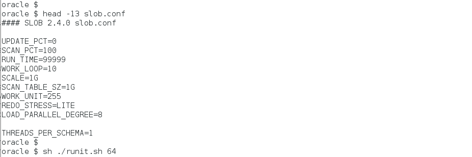
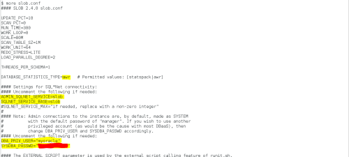
The following screenshot shows the slob.conf I used. You’ll notice that I loaded a “scan table” of 1GB for each schema. Not shown is the fact that I loaded 64 schemas.

For this type of testing I used the SLOB “batch” approach as opposed to a fixed-time test.  As Figure 1 shows, I set the WORK_LOOP parameter to 10, which establishes that each of the sessions will perform 10 iterations of the “work loop”–a “batch” of work as it were. To make the SLOB test perform nothing but table scans, I set SCAN_PCT to 100 and UPDATE_PCT to 0.

Figure 1: SLOB Configuration File.

The runit.sh script produces both the RAC and non-RAC flavor of AWR report in compressed HTML format. The files are called awr.html.gz awr_rac.html.gz.

The RAC report differs from the non-RAC AWR report in both obvious and nonobvious ways. Obviously, a RAC report includes per-instance statistics for multiple instances, however, the RAC report also includes categories of statistics not seen in the non-RAC report. It is, in fact, one of the classes of statistics–only present in the RAC AWR report–that causes the confusion for so many DBAs.

Understandable Confusion – Words Matter!

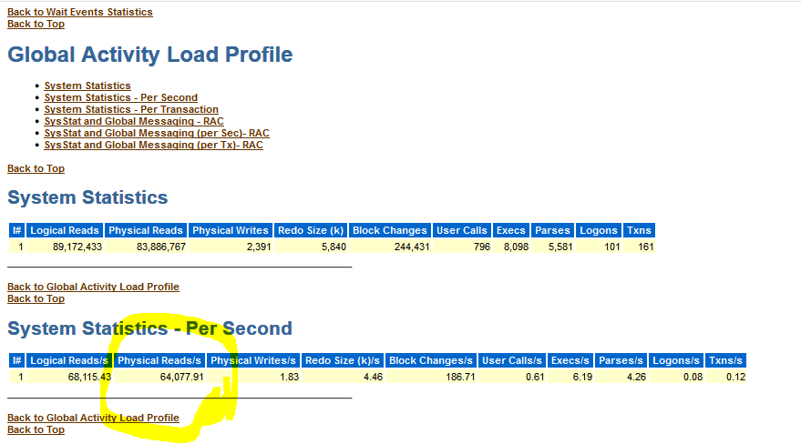
Figure 2 shows a snippet of the RAC AWR report generated during the SLOB test. The screenshot shows the crux of the matter. To check on IOPS, many DBAs open the RAC AWR report and scroll to the Global Activity Load Profile where the per-second system statistics section supposedly reports physical reads per second. I’m not even going to spend a moment of your time to split the hairs that need splitting in this situation because the rest of the RAC report clarifies the erroneous column heading.

Simply put, the simple explanation for this simple problem is that Oracle simply chose an incorrect–if not simply over-simplified–column heading in this section of the RAC AWR report.

Logical and Physical I/O

Figure 2 shows the erroneous column heading. In this section of the RAC AWR report, both logical I/O and physical I/O are reported. In this context, all logical I/O in Oracle are single-block operations. What’s being reported in this section is that there were 68,115 logical reads per second of which 64,077 required a fetch from storage as the result of a cache miss. If Oracle suffers a miss on a logical I/O (which is an operation to find a cached, single block in SGA block buffer pool), the resultant action is to get that block from storage. Whether the missed block is “picked up” in a multi-block read or a single-block read is not germane in this section of the report. That said, I still think the column heading is very poorly worded. It should be “Blocks Read/s”.

Figure 2: RAC AWR Report. Global Activity Load Profile.

What are IOPS? Operations! IOPS are Operations!

That heading made me think of Charlton Heston swinging off the back of a garbage truck yelling, “It’s Operations, IOPS is Operations”. Some may get the Soylent Green reference. Enough of my feeble attempt at humor.

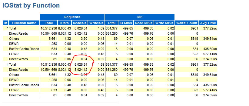
The acronym IOPS stands for I/O operations per second. The word operations is critical. An I/O operation in, Oracle database, is a system call to transfer data to or from storage. Further down in the RAC AWR is the IOStat by Function section which uses a term that maps precisely to IOPS–requests.  Another good term for an I/O operation is a request–a request of the operating system to transfer data–be it a read or a write. An operation–or a request–to transfer data comes in widely varying shapes and sizes. Figure 3 shows that the SLOB test described above actually performed approximately 8,000 requests–or, operations–per second from storage in the read path.

I’ll reiterate that. This workload performed 8,000 IOPS.

That’s a far cry less than suggested in Figure 2.

Figure 3: RAC AWR Report. IOStat by Function.

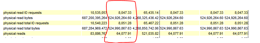
Further down in the RAC AWR report, is the Global Activity Statistics section. This section appears in both the RAC and non-RAC reports. Figure 4 shows a snippet of the Global Activity Statistics section from the RAC report generated during the SLOB. Here again we see the unfortunate misnomer of the statistic that actually represents the number of blocks retrieved from storage. Figure 4 shows the same 64,000 “physical reads” seen in Figure 2, however, there are adjacent statistics in the report to help make information out of this data. Figure 4 ties it all together. The workload performed some 8,000 read requests from storage. What was read from storage? Well, 64,000 blocks per second where physically read from storage.

Let’s Go Shopping

I have a grocery-shopping analogy in mind. Think of a requests as each time you transfer an item from the shelf to your cart. Some items are simple, single items like a bottle of water and others are multiple items in a package such as a pallet of bottled water. In this analogy, the pallet of bottled water is a multi-block read and the single bottle is, unsurprisingly, a single-block read. The physical reads statistic is the total number of water bottles–not items–placed into the cart. The number of item’s placed in the cart per second was 8,000 by way of plopping something into the cart 8,000 times per second. I hope the cart is huge.

Figure 4: Global Activity Statistics. RAC AWR Report.

As mentioned earlier in this post, the RAC AWR report is really just a multi-instance report. In this case I generated a multi-instance report that happened to capture a workload from a single-instance. That being the case, I can also read the non-RAC AWR report because it too covers the entire workload. If everyone, always, read the non-RAC AWR report there would never be any confusion about the difference between reads and payload (read requests and blocks read)–at least not since Oracle Database 11.2.0.4.

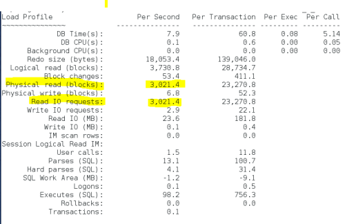
Starting in the final patchset release of 11g (11.2.0.4), the Load Profile section (which does not appear in the RAC AWR report) clearly spells out the situation with the “Physical read” misnomer. Figure 5 shows the Load Profile in the non-RAC report generated by the SLOB test. Here we can see that late in 11g there were critical, parenthesized, words added to the output. What was once reported only as “Physical reads” became “Physical read(blocks)” and the word requests was added to help DBAs determine both IOPS (requests per second are IOPS) and the payload, Again, we can clearly see that the test had an I/O workload that consisted of 8,000 requests per second for 64,000 blocks per second for a read throughput of 500MB/s.

Figure 5: Non-RAC AWR. Load Profile Section. Simple and Understandable I/O Statistics.

Wrapping It All Up

I hope a few readers make it to this point in the post because there is a spoiler alert. Below you’ll find links to the actual AWR reports generated by the SLOB test. Before you read them I feel compelled to throw this spoiler alert out there:

I set db_file_multiblock_read_count to 8 with the default Oracle Database block size.

That means processes were issuing 64KB read requests to the operating system.

With that spoiler alert I’m sure most readers are seeing a light come on. The test consists of 64 sessions performing 64KB reads. The reports tell us there are 8,000 requests per second (IOPS) and 64,077 blocks read per second for a read throughput of 500MB/s.

500MB / 8,000 == 64KB.

Links to the AWR reports:

https://github.com/therealkevinc/AWRS/blob/master/awr.html

https://github.com/therealkevinc/AWRS/blob/master/awr_rac.html

Click the following link and githup will give you a ZIPed copy of these AWR reports: https://github.com/therealkevinc/AWRS/archive/master.zip

You have applications that scan disk using large sequential reads so you take a peek at /proc/diskstats (field #4 on modern Linux distributions) before and after your test in order to tally up the number of reads your application performed. That’s ok. That’s also a good way to get erroneous data.

Your application makes calls for I/O transfers of a particular size. The device drivers for your storage might not be able to accommodate your transfer request in a single DMA and will therefore “chop it up” into multiple transfers. This is quite common with Fibre Channel device drivers where, for example, I/O requests larger than, say, 256KB get rendered into multiple 256KB transfers in the kernel.

This is not a new phenomenon. However, folks may not naturally expect how stats in /proc/diskstats reflect this phenomenon.

The following screen shot shows a simple shell script I wrote to illustrate the point I’m making. The script is very simple. As the screen shot shows, the script will execute a single dd(1) command with direct I/O for 1,000 reads of sizes varying from 4KB to 1024KB.

First, I executed the script by pointing it to a file in an XFS file system on an NVMe drive. As the next screenshot shows, diskstats accurately tallied the application reads until the I/O sizes were larger than 256KB. We can see that the device is only taking DMA requests of up to 256KB. When the script was conducting 512KB and 1024KB I/O requests the count of reads doubled and quadrupled, respectively, as per /proc/diskstats.

I’m sure readers are wondering if the file system (XFS) might be muddying the water. It is not. The following screen shot shows scanning the device directly and the resultant diskstats data remained the same as it was when I scanned a file on that device.

Summary

This was not meant to be a life-changing blog post. The main point I’m sharing is that it’s important to not confuse your I/O requests with the I/O requests of the kernel. You can scan with whatever read size you’d like. However, the kernel has to abide by the transfer size limit announced by the device driver. To that end, you have your reads and the kernel has its reads. Just remember that /proc/diskstats is tracking the kernel’s read requests–not yours.

I hope these sneak peeks are of interest…

PostgreSQL and Buffered I/O

PostgreSQL uses buffered I/O. If you want to test your storage subsystem capabilities with database physical I/O you have to get the OS page cache “out of the way”–unless you want to load really large test data sets.

Although pgio (the SLOB Method for PostgreSQL) is still in Beta, I’d like to show this example of the tool I provide for users to make a really large RAM system into an effectively smaller RAM system.

Linux Huge Pages

Memory allocated to huge pages is completely cordoned off unless a process allocates some IPC shared memory (shmget(1)).  The pgio kit comes with a simple tools called pgio_reduce_free_memory.sh which leverages this quality of huge pages in order to draw down available memory so that one can test physical I/O with a database size that is quite smaller than the amount of physical memory in the database host.

The following picture shows an example of using pgio_reduce_free_memory.sh to draw set aside 443 gigabytes of available memory so as to leave only 32 gigabytes for OS page cache. As such, one can test a pgio database of, say, 64 gigabytes and generate a tremendous about of physical I/O.

I should think this little tool could be helpful for a lot of testing purposes beyond pgio.

If you are interested in a head start on pgio, the following is a link to the full README file which has some loading and testing how-to:

The pgio text README file version 0.9 Beta

Bulk Data Loading With pgio Version 0.9 Beta

Now that pgio (the SLOB Method for PostgreSQL) is in Beta users’ hands I’m going to make a few quick blog entries with examples of pgio usage. The following are screen grabs taken while loading 1 terabyte into the pgio schemas. As the example shows, pgio (on a system with ample storage performance) can ready a 1 terabyte data set for testing in only 1014 seconds (roughly 3.5TB/h loading rate).

$ cat pgio.conf
UPDATE_PCT=0
RUN_TIME=120
NUM_SCHEMAS=4
NUM_THREADS=2
WORK_UNIT=255
UPDATE_WORK_UNIT=8
SCALE=1G

DBNAME=pg10
CONNECT_STRING=”pg10″

CREATE_BASE_TABLE=TRUE

$ echo ”
> UPDATE_PCT=0
> RUN_TIME=120
> NUM_SCHEMAS=64
> NUM_THREADS=16
> WORK_UNIT=255
> UPDATE_WORK_UNIT=8
> SCALE=16G
> DBNAME=pg10
> CONNECT_STRING=\”pg10\”
> CREATE_BASE_TABLE=TRUE ” > pgio.conf
$
$ sh ./setup.sh

Job info: Loading 16G scale into 64 schemas as per pgio.conf->NUM_SCHEMAS.
Batching info: Loading 16 schemas per batch as per pgio.conf->NUM_THREADS.
Base table loading time: 23 seconds.
Waiting for batch. Global schema count: 16. Elapsed: 0 seconds.
Waiting for batch. Global schema count: 31. Elapsed: 243 seconds.
Waiting for batch. Global schema count: 46. Elapsed: 475 seconds.
Waiting for batch. Global schema count: 61. Elapsed: 697 seconds.
Waiting for batch. Global schema count: 64. Elapsed: 935 seconds.

Group data loading phase complete. Elapsed: 1014 seconds.
$
$ psql pg10
psql (10.0)
Type “help” for help.

pg10=# \d+
List of relations
Schema | Name | Type | Owner | Size | Description
——–+——————+——-+———-+————+————-
public | pgio1 | table | postgres | 16 GB |
public | pgio10 | table | postgres | 16 GB |
public | pgio11 | table | postgres | 16 GB |
public | pgio12 | table | postgres | 16 GB |
public | pgio13 | table | postgres | 16 GB |
public | pgio14 | table | postgres | 16 GB |
public | pgio15 | table | postgres | 16 GB |
public | pgio16 | table | postgres | 16 GB |
public | pgio17 | table | postgres | 16 GB |
public | pgio18 | table | postgres | 16 GB |
public | pgio19 | table | postgres | 16 GB |
public | pgio2 | table | postgres | 16 GB |
public | pgio20 | table | postgres | 16 GB |
public | pgio21 | table | postgres | 16 GB |
public | pgio22 | table | postgres | 16 GB |
public | pgio23 | table | postgres | 16 GB |
public | pgio24 | table | postgres | 16 GB |
public | pgio25 | table | postgres | 16 GB |
public | pgio26 | table | postgres | 16 GB |
public | pgio27 | table | postgres | 16 GB |
public | pgio28 | table | postgres | 16 GB |
public | pgio29 | table | postgres | 16 GB |
public | pgio3 | table | postgres | 16 GB |
public | pgio30 | table | postgres | 16 GB |
public | pgio31 | table | postgres | 16 GB |
public | pgio32 | table | postgres | 16 GB |
public | pgio33 | table | postgres | 16 GB |
public | pgio34 | table | postgres | 16 GB |
public | pgio35 | table | postgres | 16 GB |
public | pgio36 | table | postgres | 16 GB |
public | pgio37 | table | postgres | 16 GB |
public | pgio38 | table | postgres | 16 GB |
public | pgio39 | table | postgres | 16 GB |
public | pgio4 | table | postgres | 16 GB |

The pgio kit is the only authorized port of the SLOB Method for PostgreSQL. I’ve been handing out Beta kits to some folks already but I thought I’d get some blog posts underway in anticipation of users’ interest.

The following is part of the README.txt for pgio v0.9 (Beta). SLOB users will find it all easy to understand. This is the section of the README that discusses pgio.conf parameters:

UPDATE_PCT

The percentage of SQL that will be UPDATE DML

RUN_TIME

runit.sh run duration in seconds

NUM_SCHEMAS

pgio data is loaded into either a big single schema or multiple. NUM_SCHEMAS directs setup.sh to create and load NUM_SCHEMAS schemas.

NUM_THREADS

For setup.sh:  This parameter controls the number of concurrent
data loading streams.

For runit.sh:  This parameter controls how many sessions will attach to
each NUM_SCHEMAS schema.

For example, if NUM_SCHEMAS is set to 32 and NUM_THREADS is set
to 8, setup.sh will load data into 32 schemas in batches of
8 concurrent data loading streams. On the other hand, if set to the
same 32 and 8 respectively for NUM_SCHEMAS and NUM_THREADS then
runit.sh will run 8 sessions accessing each of the 32 schemas for a
total of 256 sessions.

WORK_UNIT

Controls the bounds of the BETWEEN clause for each  SELECT statement as it executes. For example, if set to 255 each SELECT will visit 255 random blocks. Smaller values require more SQL executions to drive the same IOPS.

UPDATE_WORK_UNIT

The UPDATE DML corollary for WORK_UNIT. This allows for a mixed SELECT/UPDATE workload where SELECT statements can visit more blocks than UPDATES.

SCALE

The amount of data to load into each schema. Values can be N as a number of 8KB blocks or N modified with [MG] for megabytes or gigabytes. For example, if set to 1024 setup.sh will load 8MB  ( 1024 * 8192 bytes) into each schema whereas set to 1024M will load  1024 megabytes into each schema.

DBNAME

The PostgreSQL database that holds the pgio objects

CONNECT_STRING

This parameter is passed to the psql command. The pgio kit expects that .pgpass and all other authentication is configured. For example, if CONNECT_STRING is set to “pg10” then the following command must succeed in your pgio environment:

$ psql pg10

CREATE_BASE_TABLE

The loader, setup.sh, creates a dense “seed” table as the source from  which to load the test tables. This seed table persists after setup.sh exits. If this parameter is set to true the seed table will not be regenerated.

This is a quick blog entry to announce that the SLOB distribution will no longer be downloadable from Syncplicity. Based on user feedback I have switched to making the kit available on GitHub. I’ve updated the LICENSE.txt file to reflect this distribution locale as authorized and the latest SLOB version is 2.4.2.1.

Please visit kevinclosson.net/slob for more information.

This is just a quick blog entry to share a good paper on migrating Oracle Database workloads to Amazon Web Services EC2 instances running Oracle Linux.

Please click the following link for a copy of the paper:  Click Here.

This is just a quick blog post to inform readers of a good paper that shows some how-to information for benchmarking Amazon Aurora PostgreSQL. This is mostly about sysbench which is used to test transactional capabilities.

As an aside, many readers my have heard that I’m porting SLOB to PostgreSQL and will make that available in May 2018. It’ll be called “pgio” and is an implemention of the SLOB Method as described in the SLOB documentation. Adding pgio, to tools like sysbench, rounds-out the toolkit for testing platform readiness for your PostgreSQL applications.

To get a copy of the benchmarking paper, click here.

If It Looks Like NVMe And Tastes Like NVMe, Well…

As users of the new Amazon EC2 C5 and M5 instance types are noticing, Amazon EBS volumes attached to C5 and M5 instances are exposed as NVMe devices. Please note that the link I just referred to spells this arrangement out as the devices being “exposed” as NVMe devices. Sometimes folks get confused over the complexities of protocol, plumbing and medium as I tend to put it. Storage implementation decisions vary greatly. On one end of the spectrum there are end-to-end NVMe solutions. On the other end of the spectrum there are too many variables to count. One can easily find themselves using a system where there interface for a device is, say, NVMe but the plumbing is, for example, ethernet. In fact, the physical device at the end of the plumbing might not even be an NVMe device but, instead, a SCSI (SAS/SATA) device and somewhere in the plumbing is a protocol engine mapping NVMe verbs to SCSI command blocks.

Things can get confusing. It is my hope that someday a lone, wayward, Googler might find this blog post interesting and helpful.

An Example

Consider Figures 1 and 2 below. In each screenshot I use dmidecode(8) to establish that I’m working with two different systems. Next, I used hdparm(8) on each system to get a quick read on the scan capability of the /dev/nvme1n1 device. As seen in figure 1,  scanning the NVMe interface (/dev/nvme1n1 ) yielded 213 megabytes per second throughput. On the other hand, Figure 2 shows the nvme1n1 interface on the i3 instance delivered a scan rate of 2175 megabytes per second.

Both of these devices are being accessed as NVMe devices but, as the results show, the c5 is clearly not end-to-end NVMe storage.

Figure 1: c5 Instance Type.

Figure 2: i3 Instance Type.

Ask The Device What It (Really) Is

Figures 3 and 4 show how to use lsblk(8) to list manufacturer supplied details about the device dangling at the end of a device interface. As the screenshots show, the c5 instance accesses EBS devices via the NVMe block interface whereas in the i3 case it is a true NVMe device being accessed with the NVMe block interface.

Figure 3: Using lsblk(8) On a c5 Instance

Figure 4: Using lsblk(8) On An i3 Instance

What Kind Of Instance?

Figure 3 shows another thing users might find helpful with these new instance types based on the new Nitro hypervisor.  Now the instance type is listed when querying the Product Name field from dmidecode(8) output.

Summary

Remember storage consists of protocol, plumbing and medium.

This is just a quick blog entry to direct readers to an article I recently posted on the AWS Database Blog. Please click through to give it a read: https://aws.amazon.com/blogs/database/testing-amazon-rds-for-oracle-plotting-latency-and-iops-for-oltp-io-pattern/.

Thanks for reading my blog!

Good grief. This is short and sweet, I know, but this installment in the Little Things Doth Crabby Make series is just that–short and sweet. Or, well, maybe short and sour?

Not root? Ok, yum(8), spew out a bunch of silliness at me. Thanks.

Sometimes, little things doth, well, crabby make!

Hey, yum(8), That is Ridiculous User Feedback

Before I offer the Step-By-Step guide, I feel compelled to answer the question that some exceedingly small percentage of readers must surely have in mind–why test with SLOB? If you are new to SLOB (obtainable here) and wonder why anyone would test platform suitability for Oracle with SLOB, please consider the following picture and read this blog post.

SLOB Is How You Test Platforms for Oracle Database.

Simply put, SLOB is the right tool for testing platform suitability for Oracle Database. That means, for example, testing Oracle Database I/O from an Amazon RDS for Oracle instance.

Introduction

This is a simple 9-step, step-by-step guide for installing, loading and testing a basic SLOB deployment on a local server with connectivity to an instance of Amazon RDS for Oracle in Amazon Web Services. To show how simple SLOB deployment and usage is, even in a DBaaS scenario, I chose to base this guide on a t2.micro instance. The t2.micro instance type is eligible for free-tier usage.

Step One

The first step in the process is to create your t2.micro Amazon Web Services EC2 instance. Figure 1 and Figure 2 show the settings I used for this example.

Figure 1: Create a Simple t2.micro EC2 Instance

Figure 2: Configure a Simple EC2 Instance

Step Two

Obtain the SLOB distribution file from the SLOB Resources Page. Please note the usage of the md5sum(1) (see Figure 3) command to verify the contents are correct before performing the tar archive extraction. You’ll notice the SLOB Resources Page cites the check sums as a way to ensure there is no corruption during downloading.

After the tar archive is extracted, simply change directories into the wait_kit directory and execute make(1) as seen in Figure 3.

Figure 3: Install SLOB. Create Trigger Mechanism.

Step Three

In order to connect to your Amazon RDS for Oracle instance, you’ll have to configure SQL*Net on your host. In this example I have installed Oracle Database 11g Express Edition and am using the client tools from that ORACLE_HOME.

Figure 4 shows how to construct a SQL*Net service that will offer connectivity to your Amazon RDS for Oracle instance. The HOST assignment is the Amazon RDS for Oracle endpoint which can be seen in the instance details portion of the RDS page in the AWS Console. After configuring SQL*Net it is good to test the connectivity with the tnsping command–also seen in Figure 4.

Figure 4: Configure Local Host SQL*Net tnsnames.ora File.

Step Four

As per the SLOB documentation you must create a tablespace in which to store SLOB objects. Figure 5 shows how the necessary Oracle Managed Files parameter is already set in the Amazon RDS for Oracle instance. This is because Amazon RDS for Oracle is implemented with Oracle Managed Files.

Since the Oracle Managed Files parameter is set the only thing you need to do is execute the ~SLOB/misc/ts.sql SQL script. This script will create a bigfile tablespace and set it up with autoextend in preparation for data loading.

Figure 5: Create a Tablespace to House SLOB Table and Index Segments.

Step Five

This step is not absolutely necessary but is helpful. Figure 6 shows the size of the database buffers in the SGA (in bytes). The idea behind generating SLOB IOPS is to have an active data set larger than the SGA. This is all covered in detail in the SLOB documentation.

Once you know the size of your SGA database buffer pool you will be able to calculate the minimum number of SLOB schemas that need to be loaded. Please note, SLOB supports two schema models as described in the SLOB documentation. The model I’ve chosen for this example is the Multiple Schema Model. By default, the slob.conf file has a very small SCALE setting (80MB). As such, each SLOB schema is loaded with a table that is 80MB in size. There is a small about of index overhead as well.

Since the default slob.conf file is configured to load only 80MB per schema, you need to calculate how many schemas are needed to saturate the SGA buffer pool. The necessary math for a default slob.conf (SCALE=80MB) with an SGA buffer pool of roughly 160MB is shown in Figure 6. The math shows that the SGA will be saturated with only 2 SLOB schemas loaded. Any number of SLOB schemas beyond this will cause significant physical random I/O. For this example I loaded 8 schemas as shown later in this blog post.

Figure 6: Simple Math to Determine Minimum SLOB SCALE for IOPS Testing.

Step Six

Figure 7 shows in yellow highlight all of the necessary edits to the default slob.conf file. As the picture shows, I chose to generate AWR reports by setting the DATABASE_STATISTICS_TYPE parameter as per the SLOB documentation.

In order to direct the SLOB test program to connect to your Amazon RDS for Oracle instance you’ll need to set the other four parameters highlighted in yellow in Figure 7. This is also covered in the SLOB documentation. As seen in Figure 4, I configured a SQL*Net service called “slob”. To that end, Figure 7 shows the necessary parameter assignments.

The bottom two parameters are Amazon RDS for Oracle connectivity settings. The DBA_PRIV_USER parameter in slob.conf maps to the master user of your Amazon RDS for Oracle instance. The SYSDBA_PASSWD parameter needs to be set to your Amazon RDS for Oracle master user password.

Figure 7: Edit the slob.conf File.

Step Seven

At this point in the procedure it is time to load the SLOB tables. Figure 8 shows example output of the SLOB setup.sh data loader creating and loading 8 SLOB schemas.

Figure 8: Execute the setup.sh Script to Load the SLOB Objects.

After the setup.sh script exits, it is good practice to view the output file as per setup.sh command output. Figure 9 shows that SLOB expected to load 10,240 blocks of table data in each SLOB schema and that this was, indeed, the amount loaded (highlighted in yellow).

Figure 9: Examine Data Loading Log File for Possible Errors.

Step Eight

Once the data is loaded, it is time to run a SLOB physical I/O test. Figure 10 and Figure 11 show the command output from the runit.sh command.

Figure 10: Execute the runit.sh Script to Commence a Test.

Figure 11: Final runit.sh Output. A Successful Test.

Step Nine

During the SLOB physical I/O testing I monitored the throughput for the instance in the RDS page of the AWS console. Figure 12 shows that SLOB was driving the instance to perform a bit over 3,000 physical reads per second. However, it is best to view Oracle performance statistics via either AWR or STATSPACK. As an aside, the default database statistics type in SLOB is STATSPACK.

Figure 12: Screen Shot of AWS Console. RDS Performance Metrics.

Finally, Figure 13 shows the Load Profile section of the AWR report created during the SLOB test executed in Figure 10. The internal Oracle statistics agree with the RDS monitoring (Figure 12) because Amazon RDS for Oracle is implemented with the Oracle Database initialization parameter filesystemio_options set to “setall”. As such, Oracle Database uses direct and asynchronous I/O. Direct I/O on a file system ensures the precise amount of data Oracle Database is requesting is returned in each I/O system call.

Figure 13: Examine the AWR file Created During the Test.

Summary

Testing I/O on RDS for Oracle cannot be any simpler, nor more accurate than with SLOB. I hope this post convinced you of the former and testing will reveal the latter.

This is just another quick and dirty installment in the Little Things Doth Crabby Make series. Consider the man page for the colrm(1) command:

That looks pretty straightforward to me. If, for example, I have a 6-column text file and I only want to ingest from, say, columns 1 through 3,  I should be able to execute colrm(1) with a single argument: 4. I’m not finding the colrm(1) command to work in accordance with my reading of the man page so that qualifies as a little thing that doth crabby make.

Consider the following screenshot showing a simple 6-column text file. To make sure there are no unprintable characters that might somehow interfere with colrm(1) functionality I also listed the contents with od(1):

Next, I executed a series of colrm(1) commands in an attempt to see which columns get plucked from the file based on different single-argument invocations:

Would that make anyone else crabby? The behavior appears to me very indeterminate to me and that makes me crabby.

Thoughts? Leave a comment!